by Satoshi Miyauchi, JP1SCQ, with Nick Hall-Patch, VE7DXR
Introduction
In early November 2025, several members of our Totsuka DXers Circle in Japan (TDXC https://www.tdxc.net/abouttdxc/ ) traveled from the Tokyo area to Tanohata village in Iwate prefecture on northern Honshu island in order to take part in a medium wave (MW) DXpedition that took place on the 8th and 9th of the month. The site was about 500m (1/3 mile) from the Pacific Ocean, overlooking Kitayamazaki cliffs, a very scenic area (Figure 1), but also one from which a great deal of long-haul DX had been heard in the past, including trans-polar WBZ-1030kHz, as well as the farthest possible Antipodes DX such as R. Nacional in Argentina on 870kHz and Radio Monte Carlo in Uruguay on 930kHz.

Figure 1
Our listening post was a meeting room in the Tanohata Nature Training Center, where we set up our receivers, such as Perseus and Airspy HF+discovery, plus our recording gear and accessories (Figure 2).
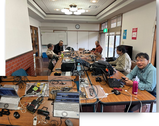
Figure 2
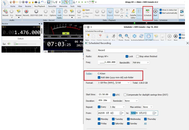
My recording software was SDR Console, but playback and analysis also used WavViewDX. We set up a TDDF (Twisted Double Delta Flag) antenna with a northeast directional pattern in order to receive medium-wave broadcasts from North America. (Figure 3)
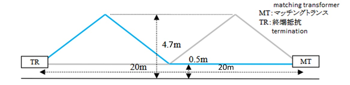
Figure 3 – TDDF antenna; note that low-noise pre-amplifier with bias-T is a must.
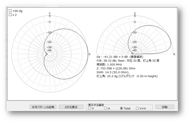
Directional patterns from Kazu GOSUI
On the second evening, November 9th, while enjoying the reception, an emergency earthquake alert was issued, and shaking struck. Inside our building, nearly 200 meters above sea level on the solid bedrock of Kitayamazaki, the shaking felt less intense than the reported magnitude of 6.9, even with an epicenter only 140km away. (Figure 4)
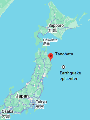
Figure 4
However, since earthquakes had been occurring even before that day and numerous aftershocks were felt afterward, it left us with a vague sense of unease. Later, a tsunami advisory was announced on the radio, plus the Tohoku Shinkansen train back to Tokyo had also stopped, and I myself couldn’t help worrying about whether it might affect my return home the following day. At that moment, I had a conversation with the members there, thinking, “If there’s something related to the earthquake recorded, that would be amazing.” However, during the real-time reception, we were targeting signals from North America in 10kHz steps, and there was no effect noticed upon those receptions.
Unusual Signal Dropouts Observed
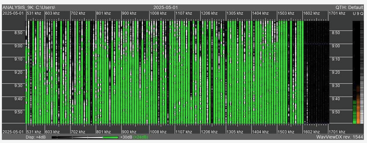
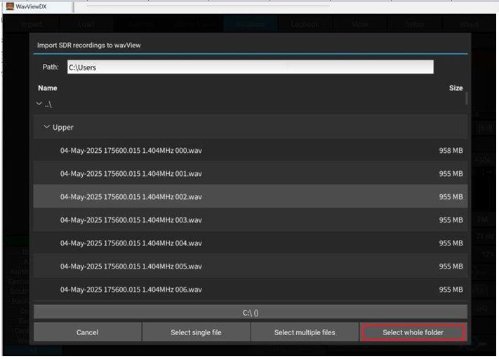
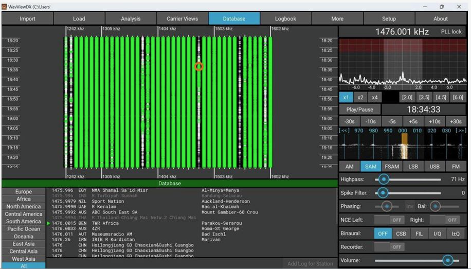
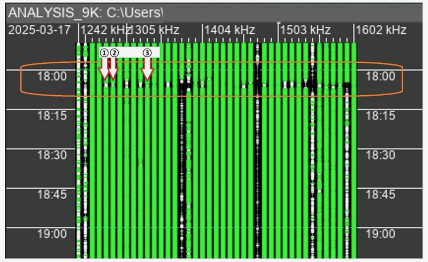
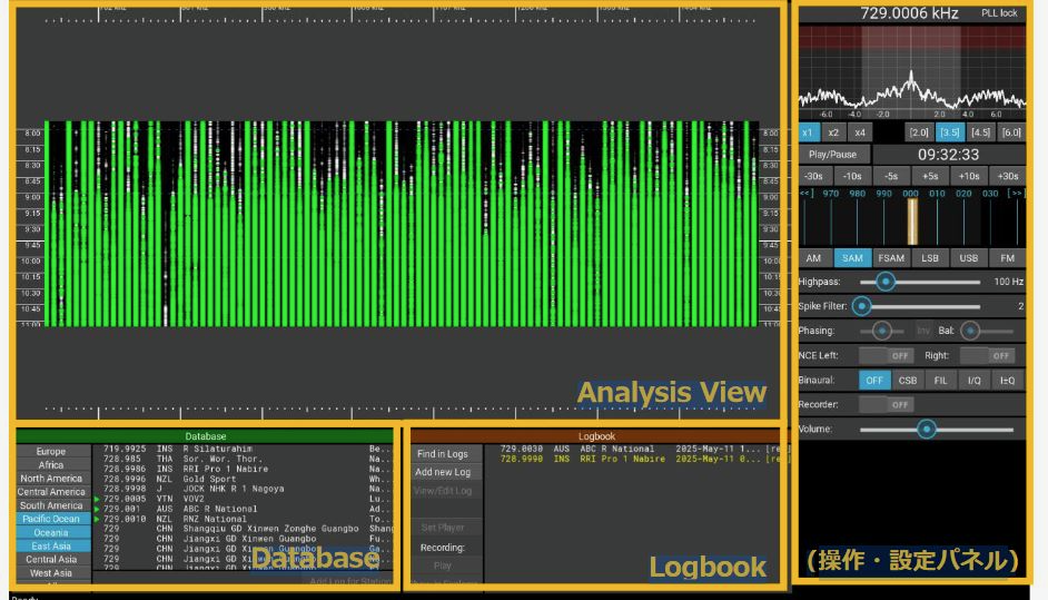
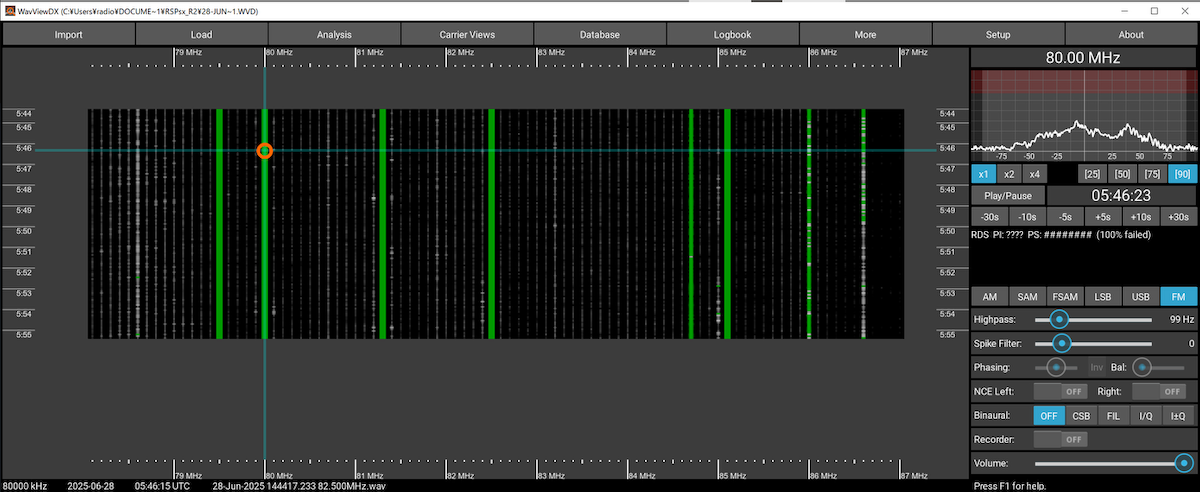
I played back the SDR files using WavViewDX (https://rweiss.de/dxer/tools.html), a software with many capabilities, including a choice of displaying all signals across the MW band at 9 or 10kHz channel spacing, but, because I was looking for North American DX, I only realized a week after returning home that the reception conditions for the 9kHz spaced domestic Japanese stations had significantly changed around 0715 to 0745UT (16:15 to 16:45 Japan time) on 9 November, based on our recordings. The dropouts on various channels over 0715 to 0745UT are quite obvious in Figure 5; I had never seen such sudden attenuation before. For those not familiar with WavViewDX, the green vertical lines on the display represent stronger signals being received on broadcast channels, while gray or black areas represent weak or no signal. (For a more detailed description of WavViewDX and its capabilities, see https://swling.com/blog/2025/10/an-introduction-to-wavviewdx-sdr-playback-software-a-totsuka-dxers-circle-article-by-kazu-gosui
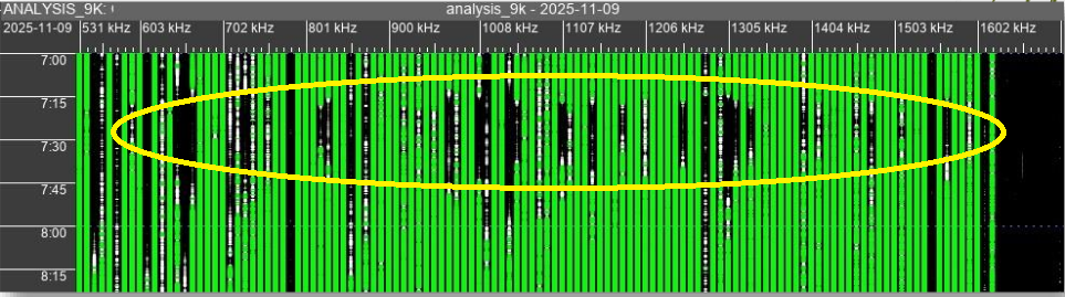
Figure 5 – WavViewDX display of signal dropouts. X-axis is frequency of received signal, Y-axis is time UTC
A first look at the data led to a couple of other observations:
- Signals originating north of the receiving site, primarily from the island of Hokkaido, were largely unaffected by the attenuation. (It is true that our antenna’s directionality was northeast, but it also received the stronger domestic stations from southwest of the antenna.)
- Regarding signals from North America, even during the same time period, the intense attenuation observed in domestic stations was generally not seen. It is unclear, however, whether some dips in North American signals around that time were due to normal fading or to the same cause that brought about the attenuation in domestic stations.
What Could Have Caused These Dropouts?
Local sunset?
These sudden drops in signal strength corresponded quite closely with local sunset at 0722UT, normally a time of disturbed propagation (see Figure 6), so the most straightforward possibility is simply the well-known change in ionospheric propagation conditions that occurs at sunset. Was that all that there was to it? However, we had been listening and recording the previous day as well, and analyzing those recordings with WavViewDX yielded no sign of dropouts in domestic signal strength at sunset on that day. Examining recordings that had been made at the same site, using similar equipment, on 24 October 2024, also showed no dropouts taking place at local sunset.
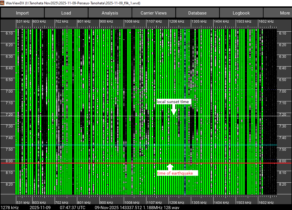
Figure 6
In fact, over many years in Japan, not only at this location but across various areas, records have been accumulated during the same time window, because good trans-Pacific DX occurs around local sunset. Nowhere in these records has a situation such as observed this time—a significant attenuation of domestic stations at local sunset—been found. Therefore, it seemed unlikely that sunset was the cause of the dropouts, but what else could it have been? Continue reading