Many thanks to SWLing Post contributor, Bob Colegrove, who shares the following guest post:
What’s Your Favorite Corner of the Dial?
As asked by Bob Colegrove
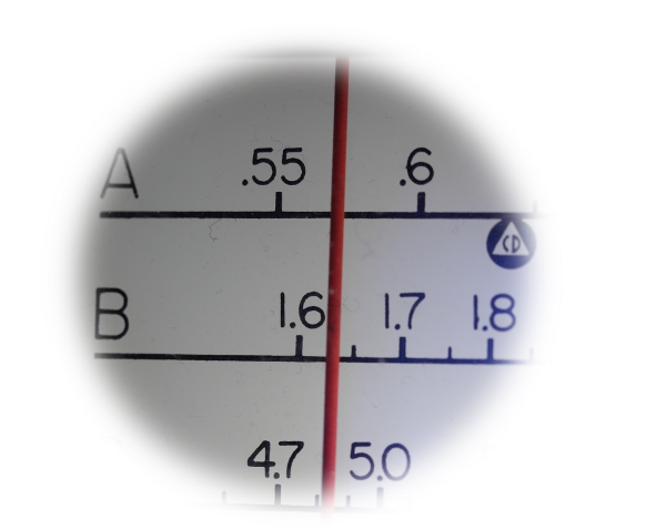
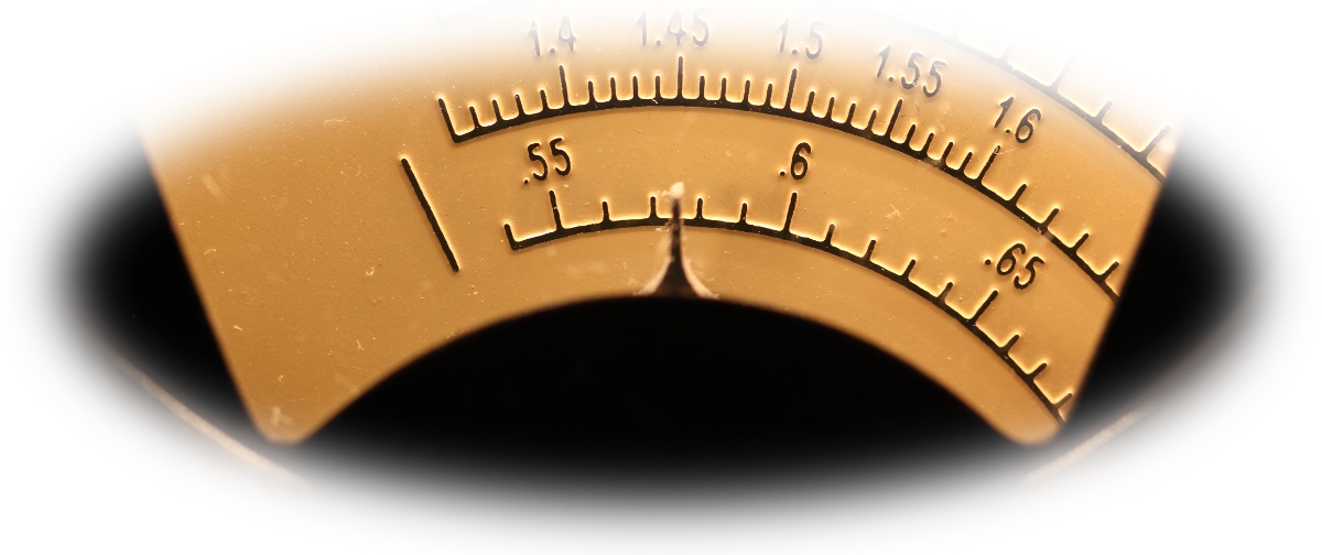 Let’s suppose you’ve been listening to radio for a while. Consciously or not, you’ve probably favored a range of AM, SW, or FM frequencies. These are areas where you go to DX or just listen to your favorite stations. One area I seem to keep returning to is the very bottom of the medium wave band, roughly 530 kHz to 600 kHz. With the convenience of today’s digital radios, I have consciously pushed the envelope somewhat lower.
The main reason for specializing in that frequency range is the challenge. In the very beginning there didn’t seem to be much at the extreme lower end of the AM broadcast band. Growing up in Indianapolis in the ‘50s, the local stations were all at the upper end of the mediumwave dial. WXLW held down 950 kHz – lower than that nothing. I would say the stator plates on the variable capacitor got very dusty, never being closed any further than that on many radios.
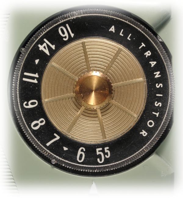
Another challenge was sensitivity. In analog times, the sensitivity of a tuned circuit had some falloff as the inductance/capacitance (L/C) ratio decreased. Sensitivity is highest with the variable cap open at the high end of the band. As you tune lower by increasing capacitance (inductance remaining constant), the Q and consequently sensitivity drop off – not dramatically, but somewhat.
Finally, not all old analog radios tuned to 530 kHz; some were even challenged to tune 540 kHz. By performing a little mischief with the alignment, I could sometimes venture into unknown territory.
This was all part of the challenge. So, what could I do to coax some activity out of the bottom of the band? I spent many hours poring over Bill Orr’s Better Shortwave Reception (Radio Publications, Inc., Wilton, CT, First Edition, 1957) and tweaking caps and coils trying to squeeze the last few kilohertz and microvolts out of my radios. This exercise fascinated me and became a hobby within a hobby. If I may be allowed a self-deprecating aside here, the first time I took a radio out of the cabinet, I just assumed that all these alignment screws were loose, and dutifully torqued them down. The alignment problem is not comparatively complex with today’s digital receivers. Note, I didn’t say it was unimportant.
 I still tend to favor the bottom of the medium wave band. Below is a list of my catches over the past couple of years. It’s just a sample of what one might hear by casual listening over time. Highlighted stations are heard during daylight hours. This is NOT intended to impress anyone, rather it is hopefully a stimulus for your own efforts.
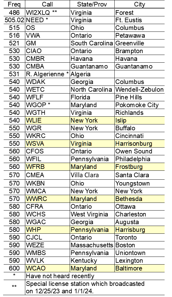 As another attraction of the lower mediumwave band, you will find a potpourri of stations. Besides regular North American broadcasting stations, one might possibly hear an occasional high-powered trans-Atlantic station which is not synchronized with the 10 kHz spacing. 530 kHz is interesting. It is not used in the US by commercial broadcast stations. Instead, stations from Canada and Cuba at roughly orthogonal directions from me are regularly audible at night on this frequency. Thus, the radio is tuned by simply rotating the antenna. 530 kHz is also home to several Travelers’ Information Stations (TIS) throughout the country. Question: How will this long-time service fare if travelers don’t have AM radios in their new cars? Finally, the very bottom of the frequency range still contains a few holdouts of non-directional beacons.
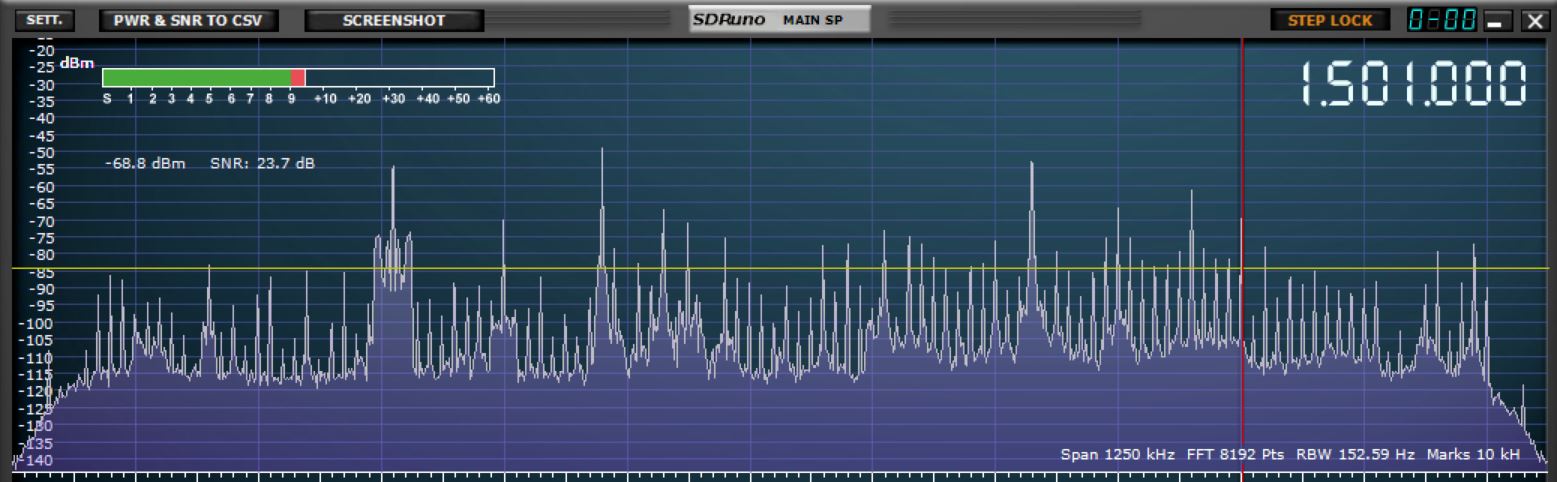
Frequencies below 530 kHz probably put a strain on the medium wave bands of old radios, but they are likely no problem on most digital radios having both LW and MW coverage. As mentioned, there are a few non-directional beacons down there. They are Morse coded using amplitude modulation. I have found placing the receiver in SSB mode makes detection much easier, as the heterodyne from the carrier can be heard well before the signal is strong enough to produce any audio. These beacons generally fade in for brief periods of time and then fade out like passing comets.
 My most recent catch was experimental station WI2XLQ, 486 kHz, during its annual Fessenden Event on Christmas Day and again on New Year’s Day. See https://swling.com/blog/?s=Fessenden+ . The experience was not the armchair listening quality one might expect from FM or the Internet. Instead, it was weak and fraught with atmospheric noise. The station came in periodically, then disappeared, in short, DXing to its highest degree of satisfaction.
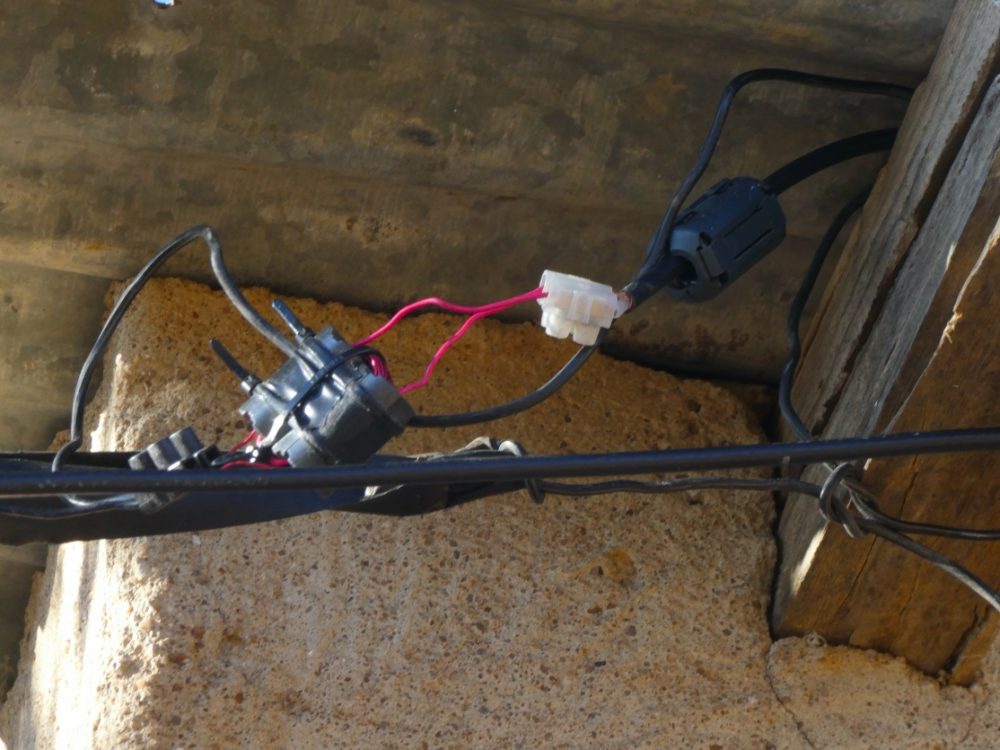
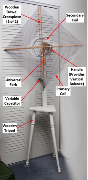
The antenna is the key to good reception, and there is no exception to this rule at the lower end of the AM band. Many years ago, I switched to an indoor, resonant loop antenna. The selectivity, directional properties, and noise rejection of a loop antenna in this frequency range are superb. The figure below shows my 40-year-old loop antenna, which is still used in its original form. It tunes from ~485 kHz through ~1710 kHz in two bands. The antenna can rotate 360 degrees horizontally and 90 degrees vertically. Further, it is mechanically balanced to remain in any position without locking. For those not inclined to construction projects, the Tecsun AN-100, AN-200, and Terk Advantage will perform quite well through inductive coupling with a portable radio’s ferrite bar antenna.
 As all experienced medium wave DXers know, for success you need to have patience, “set a spell,” and let the radio do its thing. Radios are living organisms, kind of like cats, very independent at times, and will let you hear only what they want you to hear. On many channels, stations will come and go over time. If you’re lucky, you might catch an ID; lacking that, you might be able to identify it by the format or network. You might try to compare the contents you hear on the radio with what you can hear online either over the station’s website or via streaming sites such as TuneIn, iHeart, or Radio Garden. There may be a delay between the Internet stream and the live signal.
When you feel you’ve exhausted the possibilities, there’s still more. Turn the antenna 90 degrees and start over. You’re only half finished with that frequency. Don’t forget a headset or earbuds.
What’s the next challenging rung on the limbo bar? Well, possibly the 633-meter ham band, 472 to 479 kHz. I’ll have to pad the old loop with a small capacitor to tune down there.
What’s your favorite corner of the dial? Why?