Tag Archives: Propagation

Meteor Scatter with WSJT-X

(This is an article from the August 2023 edition of The Spectrum Monitor, used with the kind permission of Ken Reitz, editor — Robert Gulley, K4PKM)

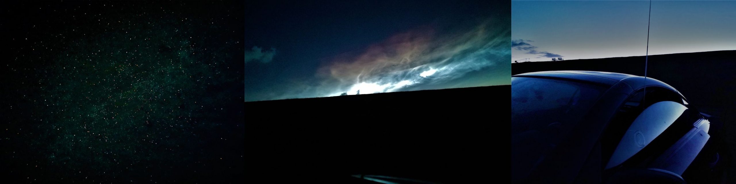
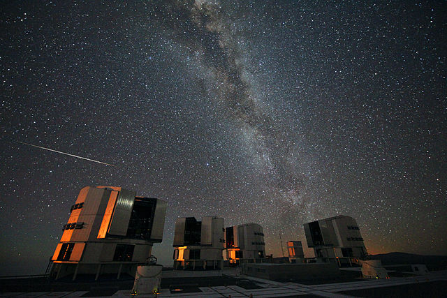
Perseid meteor streak. (Courtesy: European Southern Observatory, via Wikimedia creative commons)

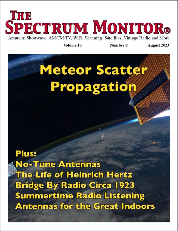
Incoming! An Introduction to Meteor Scatter Propagation
By Robert Gulley K4PKM

One of my all-time favorite quotes from Shakespeare comes from Hamlet: “There are more things in heaven and earth, Horatio, than are dreamt of in your philosophy.” When I first heard about bouncing a signal off the moon and back to earth I thought “how can that be?”
Then I heard some German folks had bounced a signal off Venus and received it back. “How can that possibly happen?” Indeed, there are more things in heaven and earth than are dreamt of in my philosophy! Enter Meteor Scatter.

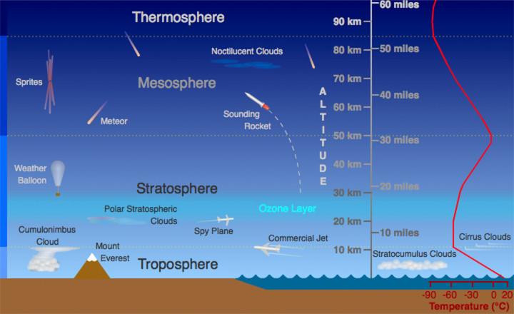
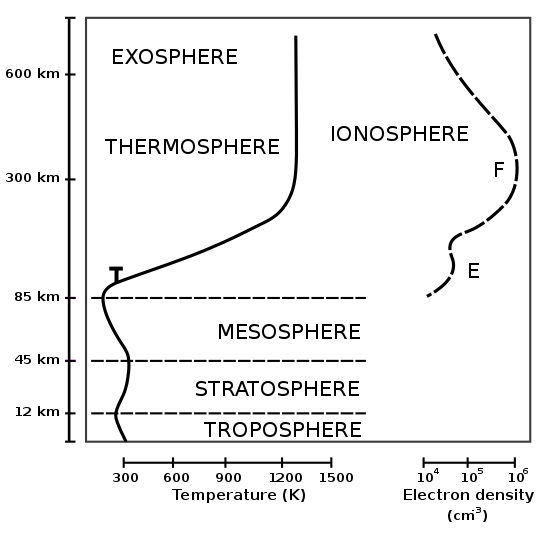
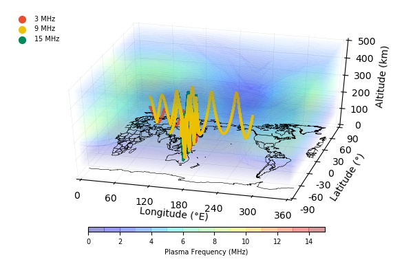
Meteor Scatter is a propagation phenomenon where signals sent up into the atmosphere are reflected back down to earth by the ionization trails left by meteors as they cross our skies. As the meteors move through the atmosphere, they heat up vapor particles which can then reflect VHF and UHF signals in irregular patterns. These trails typically only last for a few milliseconds up to a few seconds, but with modern digital software, that’s enough time for a lot of information to be passed along. This occurs in the “E” layer of the atmosphere.

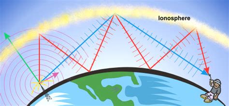
Likely you have heard of E-skip propagation, where VHF (and occasionally UHF) signals can travel much further than the typical line-of-sight propagation. Meteor scatter works similarly to allow much greater DX distances, typically up to 1000 or so miles, and occasionally even greater distances. Similar to other propagation modes, meteor scatter can occur as forward or backward scatter.

What’s even more exciting, it does not take a super-station to hear or make these contacts! An
antenna and radio capable of receiving 6-meter signals will work just fine with the right software. Radios that can receive 6 meters can have their audio sent to WSJT-X software using the MSK144 mode to listen in, and amateur radio operators can transmit using typical radio output power to either a 6-meter vertical or horizontal dipole. While a directed antenna will produce the best results, the variable nature of the reflected signals makes almost any antenna capable of 6-meter reception/transmission useable.

Unlike line-of-sight propagation which typically works best with matching polarization, there is no one pattern to meteor scatter. Elevation, meteor trail direction, location of stations, forward vs. backward scatter, all are variables that make working meteor scatter more fun and more frustrating!

As an aside, working distances of 1200 miles or so is considered DX on 6 meters, and definitely on 2 meters and above. DX is relative to the band and mode being used, not strictly working other countries. Where I live, 1200 miles is excellent, but won’t take me to Europe or over into the Pacific. However, the DX is just as exciting knowing I am pushing the limits of a given mode and frequency combination.

A Little History

In 1929 a Japanese scientist, Hantaro Nagaoka, first suggested observable propagation from meteors in a paper entitled: Possibility of the Radio Transmission being disturbed by Meteoric Showers. By the 1940s, meteor scatter was further established by Stanley Hey, a British physicist and radio astronomer. His work during WWII with radar led directly to discoveries of both meteor scatter and radio waves coming from the sun and other galaxies. I highly recommend reading about him!

Having close ties to military research, it was not long before the military started using meteor scatter as a means of long-range communication by the 1950s. Canadians developed a meteor scatter program called JANET. A NATO document from December 6, 1961, requests information on communications via “meteor trails.” NATO’s Supreme Headquarters Allied Powers Europe
developed a program of meteor scatter communications called COMET (COmmunication by MEteor Trails), with stations in the Netherlands, France, Italy, West Germany, the United Kingdom, and Norway. With the introduction of satellites, meteor scatter communications took a backseat, as satellite communications were assumed to be more reliable.

However, due to vulnerabilities of satellite communications being intercepted, meteor scatter has once again become a source of communication for the military as well as other governmental agencies. (This history, as well as much additional information on meteor scatter communications can be found by searching: Meteor Burst Communications: An Additional Means Of Long-Haul Communications by Major John P. Jernovics Sr., USMC.

Amateur Radio and SWL Use

Amateur radio operators have for years been using various modes to take advantage of the expanded reach meteor scatter can provide, including SSB, Morse code, and digital mode software such as WSJT-X. Before our current digital mode software, CW was in common use, where data would be sent and recorded in bursts up to 800 words per minute. Specially modified tape recorders would then play back the messages at much slower speeds to allow copying the code at normal speeds. With the advent of personal computers, this made the sending/copying process much easier.

Fortunately, today we have readily and freely available software to allow communication in real time. The wildly popular WSJT-X software by Joe Taylor has meteor scatter software built in. Using the MSK144 protocol, signals are coordinated between both sending and receiving stations to allow for the most efficient transfer of information. While listening to meteor scatter transmissions has always been possible for shortwave listeners, today’s digital software makes it incredibly easy to receive these signals and log some very interesting stations and locations. Many SDR radios are capable of 6-meter reception, as well as the 2-meter and 70-cm bands. SDRs also have the benefit of digital filtering, allowing the signals to be pulled out more
cleanly.

On the transmitting side, if you are familiar with FT8 and FT4 then switching to MSK144 will not be much of a learning curve. If you are new to WSJT-X or similar software, I would advise spending some time getting comfortable with FT8 and/or FT4 before diving into meteor scatter
work. While one does not have to know these modes to use meteor scatter, I believe it helps.

For the sake of brevity, I will assume a basic familiarity with digital modes, and concentrate on how meteor scatter works within WSJT-X.

Unlike FT8 and other standard digital modes, meteor scatter MSK144 has standard frequencies which, while not absolute, are very widely acknowledged among users. When choosing a band, the default frequencies brought up by the software should be used, unless you know for certain a station is transmitting (or listening for you) on a non-standard frequency. I recommend starting with 6 meters, as it is by far the most active. If you have 2 meter/70cm all-mode capability, wait until you are comfortable with the back-and-forth flow of contacts before moving on from 6 meters.

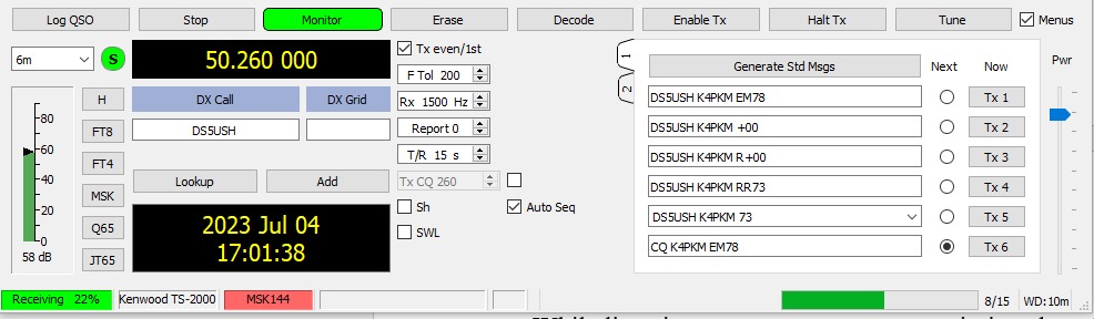
These are the recommended settings for meteor scatter mode using WSJT-X.

Notice the default settings on the WSJT-X screen for meteor scatter in the screen capture. F Tol (frequency tolerance) is set to 200, RX (Receive) is set to 1500 Hz, and Report is set to 0. I would also suggest having your radio’s pre-amp turned on for this mode. You can adjust the Fast Graph shown below) brightness through sliders on the panel or use the auto level feature.

One place where this meteor scatter protocol differs from standard FT8 or similar modes is the mutually agreed upon standard practice of stations transmitting (pointing) to the east transmit on even cycles (each cycle is 15 seconds long: 00, 15, 30, 45, 00), so they would transmit on 00 and 30 second marks, while stations transmitting (pointing) west transmit on the odd cycles (15, 45).

You will notice there is a check box for TX even/1st – stations transmitting toward the east coast would have this box checked, whereas stations trying to work to the west would leave the box unchecked. Clear as mud, right?! Perhaps an acronym will help you remember the proper sequence. PETE = Point East Transmit Even.

This is of primary importance when calling CQ. When answering a CQ call (sometimes referred to as search and pounce mode), the software will handle transmitting on the proper cycle. This is the style of operating I use most, but I do occasionally call CQ in an effort to find out if anyone can hear me. This is when I need to make sure I am following the standard protocol.

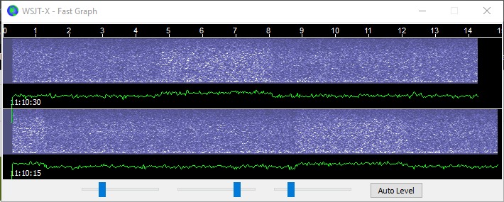
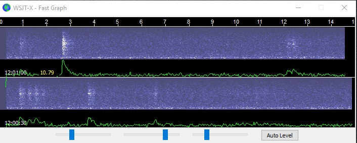
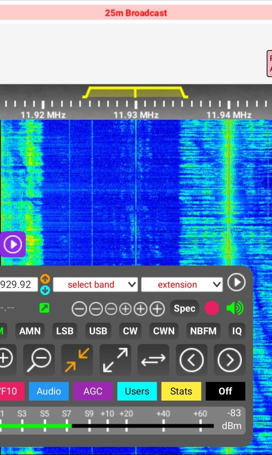
Top: The Fast Graph display shows a base level reception which can be adjusted for
brightness and contrast similar to an SDR waterfall. Bottom: Typical reception graph
with signals making vertical markings and sounds similar to static crashes.

The hardest part of working meteor scatter is waiting for a signal to show up calling CQ, or having one answer you if you are trying to initiate contact with CQ. This can take time. Remember, you are depending on wispy trails of ionization to reflect your signal to someone else on the planet, either to answer their call or reach someone with your call. Be patient! It is not uncommon for a station to call 5, 10, even 15 times before someone responds. And the waiting is not over . . . .

To complete a contact after hearing CQ, you may have to respond to that CQ call over a number of cycles before the meteor trail gods bring all those meteors into alignment so that your response reaches the person on the other end. It is not uncommon for contacts to range over 10 minutes or more. Fortunately, it is usually much less. However, this is not like a DXpedition where once you are called back the rest of the contact is over in 30 seconds.

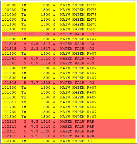
Left: While not always typical, contacts can take 10 minutes or more to complete on days when meteor activity is low; typically contacts last over several minutes or more.

In the screen capture showing a typical contact, notice I initiated my response call at 10:09:00 (as I was pointing east), and the contact continues over 36 cycles (I counted for you!) and spans 12 minutes. Now before you tune out and say “Whoa, no way, man! That’s crazy!” I have two very valid points to make. 1) If you are chasing a rare DX station as I often do, it is nothing for me to try for 20 minutes or more to break the pileup and make the contact. I have actually spent 3 hours or more attempting to work a really rare DX station. Compared to that, 5, 10, or even 15 minutes is not a long time. 2) Stop and think about how totally cool it is to be using meteors to be making a contact with someone!! That’s definitely worth some real bragging
rights to your ham buddies who have never done this, and just the cool factor alone keeps me coming back to see how far I can make a meteor scatter contact!

If you are like me, radio is still magical, and meteor scatter is all the more so – we are interacting with particles that have travelled thousands and thousands of miles to get here! That’s awe inspiring!

While perhaps not quite as amazing as bouncing your signal off the moon to contact someone halfway around the world, it is still really exciting to think you can send massive amounts of data in a short burst before a meteor trail fizzles out in a matter of seconds or less. MSK144 transmits a complete data package, including redundant data features, every 70 milliseconds!!
This is why you may see a half dozen or more repeats of a signal in the same cycle as each data package is received and decoded. The redundant nature of the transmission helps to deal with the chaotic randomness of the meteors. If even one data package gets through, then the receiving station can answer accordingly.

You might be wondering, “How can I react fast enough to respond to packets sent in 70 millisecond intervals?” You do not have to. Remember we are dealing with 15 second cycles,
so once a CQ comes through and you double click on it to respond (just as with FT8 etc.), the software does the rest, assuming Auto Sequence is checked. The software then follows the
same pattern as when making auto-sequenced FT8 or FT4 contacts. If you are calling CQ, the auto sequence is even easier once someone responds, again, just like FT8.

You can see why I said it is best to get familiar with FT8/FT4 before trying meteor scatter. You will be a lot more relaxed making these amazing contacts with some real digital mode experience to fall back on.

Strategies for Working/Catching Contacts

The best time for hearing or working other stations is during the early morning hours, typically between a little before dawn until several hours after daylight. By the time the sun comes up in your area the signals will mostly fade away as the atmosphere heats up and signals are absorbed.

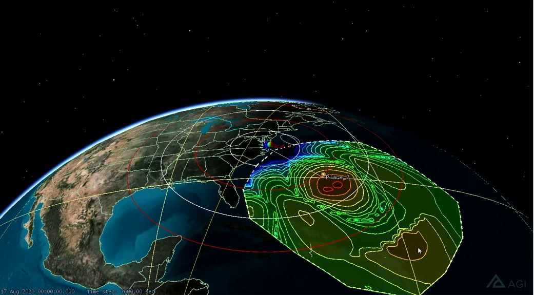
Don’t expect every day to produce lots of signals, conditions vary a great deal. As I discuss further down, there are times of high meteor activity, but most days have varying opportunities, much like normal contacts and propagation vagaries. If the atmosphere is disturbed by geomagnetic storms, solar flares, CMEs and the like, then listening conditions will be adversely affected with this mode just as with other modes. However, don’t just assume conditions will be poor based on the typical propagation reports (good advice for any mode!). Because we are dealing with extremely short data bursts, signals may come through even when conditions
seem difficult for other modes.

The main thing is to not get frustrated with trying to hear or work meteor scatter contacts. It is a very special mode, and with some experience and understanding of how the mode works, you will hear and/or make a good number of contacts over time.

Unlike FT8 or other digital modes, I turn the volume up on the radio to a reasonable level to hear the meteor signals. With FT8, FT4, JT65 or similar modes, I keep the volume off unless I am wanting to try to identify something causing interference, such as a different mode being used or something local. Meteor scatter (MSK144) signals sound like static bursts rather than the familiar tones of FT8. By having the volume turned up I am able to quickly tell when there are signals present. This allows me to do other things while monitoring the band, useful when
there are slow signal days. As a matter of fact, I am listening to the band and switching screens as needed while writing this article – actual multitasking!

Contacts are made in much the same way as other digital modes, but with a couple of notable exceptions. As shown in the screen capture with contacts happening over 9 minutes, there is often a lot of repetition. Even when signals seem strong coming into your station on the receive cycle, it does not mean the other station is going to hear your response on the next transmit
cycle.

Here’s an example of a typical contact. I hear A8XYZ sending CQ. I respond to his call on my next transmit cycle. I then hear him calling CQ again on his next transmit cycle. This may go on for several cycles or more, but since he is a new grid for me, I persist.

Finally, he responds to my call with a signal report as part of the auto sequence feature of the software, once he has heard me calling him. His computer then sends me his signal report over multiple cycles as needed until my computer sends him a RRR or RR73 depending on my settings. Since he does not receive my RR73 the first time I send it, his computer continues to send a signal report. When he finally does receive my RR73, he sends his 73 to indicate the completed contact. He likely does this for only one or two cycles because otherwise we would end up in a continuous loop of 73s back and forth.

Here’s a case where the contact was not completed, and so it is up to you and the other station as to whether the contact is confirmed.

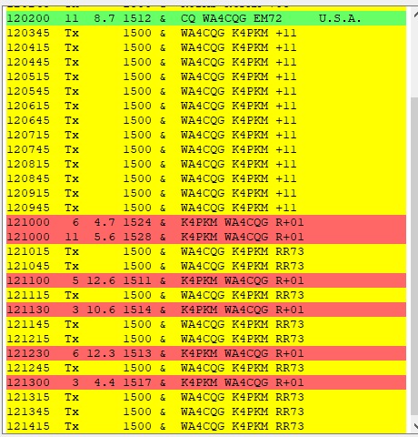
Sometimes the whole contact is over in a couple of minutes, sometimes longer. Then there are the times as indicated in the screen capture with WA4CQG, I never received a 73 from him after repeatedly sending my RR73. Since he continued to send a signal report, he does not know that I have acknowledged his signal report, and thus is not a full, standard contact.

To Confirm or not to Confirm, that is the Question!

Now, here’s the tricky part in terms of the contact with WA4CQG; technically we made a valid contact and can log it as such, even though we never got past his signal report. Since he was calling CQ, and I answered his CQ with a signal report (which he obviously received based on his then sending a signal report), that is all that is needed for a valid contact. Many people will not log it as such because they do not feel it was a full contact, but some will. Since I was sending RR73 to his signal report, my computer automatically logged the contact to my logging software, and I will upload it to LOTW and eQSL. Now it will be up to WA4CQG as to whether or not he logs the contact on his end to determine if we have a completed and confirmed QSL in our respective logs. (And yes, this is happening in real time as I write this article!)

I use this contact as an example to make an important point: just because you know it is a valid contact does not mean the other station sees it as such, and thus diplomacy is the order of the day if you choose to pursue the issue with the other station (I won’t in this case, it’s not a rare contact I need in my log). The choice to confirm the contact, and it is definitely a choice and not an obligation, rests solely in the other station’s hands.

[Additional Note: He did end up confirming the contact!]

Good operating etiquette requires that if you contact the other station requesting confirmation, you do so knowing full well it is purely the other station’s prerogative to confirm or not. I typically say something like “I show us making a contact on [date] and [time] with a signal report of [xx]. Since you apparently did not receive my 73, the call is yours as to whether or not you confirm the contact, and I will respect your decision either way. If I can provide more info, please let me know. Thank you!!” Good manners and friendly attitudes are far more important than a log entry!

Awards: If you like chasing awards, one of the more fun ones, and relatively easy to achieve over time, is the ARRL’s VUCC award for working 100 or more maidenhead grid squares. You can combine 6-meter E-skip, trans-equatorial contacts, and meteor scatter VHF contacts, as well as other VHF propagation/mode contacts for this award (but not contacts made using a repeater). If you happen to use the excellent program JTAlert, you can set alerts to indicate new
grid squares, allowing you to more quickly achieve the 100 needed grids for the award (assuming the other stations will confirm on Logbook of the World or through QSL cards).

Web Resource for Tracking/Scheduling/Posting: A great resource on the internet is Chris Cox N0UK’s site, pingjockey.net. From there you will want to go to the Ping Jockey Central page and put in your details under “User Details” where you can then read and send messages with other meteor scatter users. There is good camaraderie there, as well as the opportunity to see who’s active, and possibly set up a scheduled contact with another station. [Or, if you are just monitoring the meteor scatter frequencies, you can let folks know you have heard them, which is a big help to them.]

Additionally, while you are not allowed to short-circuit the contact process, it is common to let another station know you are receiving them and trying to call them back. This helps the other station at least know they are being heard, and they can continue to call in hopes of a contact. It also allows you or the other station to decide when to stop trying for the contact, so that neither are wasting time calling someone who has moved on.

Meteor Showers

I have saved the best for last! If you are reading this August issue as it comes out in 2023, the annual Perseids meteor shower is already underway, and is expected to peak on August 13 with up to 84 meteors per hour – that’s prime meteor scatter communication time! (As a bonus, for the purposes of viewing the Perseids, the moon will be a waning crescent, meaning a darker sky on the August 12-13).

The last several weeks of July and most of the month of August, the atmosphere will be primed for some great meteor scatter contacts. Give it a try while the “gettin’s good” as they say. And while meteors are in the sky literally every day, special times like the Perseids offer the chance to rack up a large number of contacts in a relatively short time, and that will make the experience all the more rewarding! While the Perseids are the largest meteor show, there are a number of meteor showers throughout the year. You may want to research other meteor showers and mark your calendar accordingly.

Wrap-up

Meteor scatter signals are a lot of fun to receive and to fill your logs with some very interesting contacts, whether as a shortwave listener or an amateur radio operator. With modern software the process is about as easy as one can get, and our radio forefathers would be quite jealous of our capabilities.

Something I did when starting out was to leave my radio on overnight to see what stations were being heard, and this gave me an idea of when signals were the most active. Keep in mind the various time regions and when they might start getting active or ending.

For me, in the Midwest portion of the United States, as morning comes and the sun gets stronger, I turn toward the western part of the country to try to work stations which are just approaching dawn. This allows for a longer contact period, and thus more opportunities to hear more distant stations. I believe my longest contact has been 949 miles. I can’t wait to reach over 1000!

Meteor scatter is a mode that rewards patience. Admittedly, it takes some getting used to in terms of repetition and the duration of contacts, but it is well worth the effort. Even if you only work the mode during known meteor shower opportunities, there will be many interesting contacts possible. And who knows? You may just find the mode as addicting as I have!

Robert Gulley, K4PKM, is the author of this post and a regular contributor to the SWLing Post.

Spread the radio love

You and the ionosphere: Share your propagation stories!

29 Replies

Many thanks to SWLing Post contributor, Jock Elliott, who shares the following guest post:

You and the ionosphere . . . a reader participation post

By Jock Elliott, KB2GOM

Here’s a shocker for you: we live at the bottom of the sky. Above us there are multiple layers of the atmosphere, pressing down on us at 14.7 pounds per square inch.

Of particular relevance to us as shortwave listeners and hams, there is a special layer of the atmosphere, not shown on the chart above called the ionosphere. The ionosphere starts around 30 miles above us and extends up to about 600 miles and includes parts of the layers above.

The Sun’s upper atmosphere, the corona, is very hot and produces a constant stream of Ultra-Violet and X-rays, some of which reach our atmosphere. When the high energy UV and X-rays strike the atmosphere, electrons are knocked loose from their parent atoms and molecules, creating a layer of electrons.

Now, here’s the cool part: this layer – the ionosphere – is important because radio waves bounce off of it.

The sun, however, is not constant in its action on the ionosphere. The amount of UV and x-ray energy (photon flux) produced by the sun varies at by nearly a factor of ten as the sun goes through an 11 year cycle. The density of the ionosphere changes accordingly, and so does the ability of the ionosphere to bounce radio waves. When the sun is at peak activity, and the ionosphere is “hot,” SWLs and hams are likely to experience excellent long-range propagation. When the sun is quieter, long-range propagation diminishes.

Every 11-year solar cycle is unique, but early indications are that we may on the verge a cycle that favors long-range propagation: https://swling.com/blog/2022/03/termination-event-may-indicate-solar-cycle-strength/

The results can be spectacular. Decades ago, during a particularly hot solar cycle, I once spoke from my station near Albany, NY, to a station in the state of Georgia on a mere 4 watts. On another occasion, I conversed with a ham in Christchurch, New Zealand – a distance of over 9,000 miles – with 100 watts single sideband transmit power. During that same period, I would routinely listen to shortwave stations halfway around the world.

And now, it’s your turn – what’s your favorite long-range propagation story, either as an SWL or ham? Please comment!

Spread the radio love

HF-START Web Tool: A new web-based, real-time shortwave radio propagation application

2 Replies

Many thanks to SWLing Post contributor, Tracy Wood, who shares the following journal abstract from EurekaAlert.com:

Commencement of shortwave propagation simulator (HF-START) service

Demonstrating radio wave propagation paths between any two points based on real-time space weather information

NATIONAL INSTITUTE OF INFORMATION AND COMMUNICATIONS TECHNOLOGY (NICT)

[Abstract]

The National Institute of Information and Communications Technology (NICT, President: TOKUDA Hideyuki, Ph.D.), in collaboration with Electronic Navigation Research Institute, National Institute of Maritime, Port and Aviation Technology (ENRI, Director General: FUKUDA Yutaka) and Chiba University (President: TOKUHISA Takeshi), has started the service of shortwave propagation simulator (HF-START). It provides real-time shortwave propagation that reflects real space weather information from ground-based observations and model calculations. The HF-START web system has been successfully developed and is now available at https://hfstart.nict.go.jp/.

The web calculation function of this system allows shortwave propagation between any two points in Japan based on real-time GNSS observations and between any two points on the Earth based on model-based space weather information. Real-time estimation is possible. The calculation in the past and up to about 1 day ahead in the future is also possible. In addition to amateur radio, HF-START is expected to benefit efficient frequency operation of aviation communications that relies on shortwave in the polar route.

[Background]

Communication and positioning technologies play an important role in social infrastructure in various fields today. The ionosphere has regular temporal cycles and fluctuates greatly every day associated with solar activity and space environment. Of benefit to us is the fact that ionosphere is good at refracting shortwave, which is why we can hop shortwave signals off the ionosphere to communicate with people over large distances.

Shortwave band has been used for communication and broadcasting for a long time, and are still widely used in radio broadcasting, aviation communication, amateur radio, etc. Ionospheric variation, however, has a great influence on the propagation of radio waves. Communication environment such as the communication range and usable frequency changes significantly due to the influence of the ionospheric fluctuation. Thus, fluctuations in the ionosphere affect the operation of shortwave broadcasting, aviation communications, and amateur radio.

There have been websites that provide estimated information on how radio wave propagation changes due to such ionospheric fluctuations. The problem is that it is based on a simple model and does not reflect realistic ionospheric fluctuations.

[Achievements]

We have developed a shortwave propagation simulator HF-START that estimates and provides shortwave propagation information in real-time under realistic ionospheric fluctuations based on ground-based observations and model calculations. We open real-time information estimated by HF-START, and the web application at https://hfstart.nict.go.jp/.

Figure 1 shows an example of visualization of shortwave propagation by HF-START. In this system, the user can check the radio wave propagation information that is updated in real-time. As shown in Figure 2, the user can also use the web application to estimate and visualize radio wave propagation by specifying any frequency in the range of 3-30 MHz, any two points on the Earth, and any transmission angle. The date and time can be set retroactively to the past (after 2016), to the real-time, and in the future (up to about 1 day ahead).

The system can be used to visualize the radio propagation path and clarify whether it is affected by space weather when the shortwave you are using does not reach the destination, or when you can listen shortwave broadcasted from the far source that normally you cannot hear. Furthermore, in addition to amateur radio, it is expected to benefit efficient frequency operation of the aircrafts that use shortwave in polar route.

[Future Prospects]

We are conducting research and development to extend the HF-START to estimate radio wave propagation not only in the shortwave band but also in other frequency bands. In addition, we will evaluate the simulator accuracy and improve it by comparing it with radio wave propagation observations.

NICT has been providing information related to communications, satellite positioning, and radiation exposure since November 2019 as a member of the Global Space Weather Center of the International Civil Aviation Organization (ICAO). With the HF-START service, we expect to improve the information provided to directly relate to communications, such as communication range information.

###

As the abstract mentions, you can use the tool online now via the HF-Start Web Tool.

Thanks so much for the tip, Tracy. This is fascinating!

Spread the radio love

Video demonstrating 3D propagation simulation

1 Reply

Many thanks to SWLing Post contributor, Gregory Ivanov, who writes:

Hi, found this video–I think it’s pretty cool. Shows some impressive 3D propagation simulation, I haven’t seen before:

Wow! That is fascinating. Thank you for sharing this, Gregory. 3D tools like this could be invaluable for predicting propagation even for hams and SWLs.

Of course, all of this is based on the amazing VOACAP application.

Spread the radio love

Guest Post: Why does radio reception improve on saltwater coasts?

10 Replies

Many thanks to SWLing Post contributor, 13dka, who shares the following guest post:

Gone fishing…for DX: Reception enhancement at the seaside

by 13dka

In each of my few reviews I referred to “the dike” or “my happy place”, which is a tiny stretch of the 380 miles of dike protecting Germany’s North Sea coast. This is the place where I like to go for maximum listening pleasure and of course for testing radios. Everyone knows that close proximity to an ocean is good for radio reception…but why is that? Is there a way to quantify “good”?

Of course there is, this has been documented before, there is probably lots of literature about it and old papers like this one (click here to download PDF). A complete answer to the question has at least two parts:

1. Less QRM

It may be obvious, but civilization and therefore QRM sources at such a place extend to one hemisphere only, because the other one is covered with ocean for 100s, if not 1000s of miles. There are few places on the planet that offer such a lack of civilization in such a big area, while still being accessible, habitable and in range for pizza delivery. Unless you’re in the midst of a noisy tourist trap town, QRM will be low. Still, you may have to find a good spot away from all tourist attractions and industry for absolutely minimal QRM.

My dike listening post is far enough from the next small tourist trap town (in which I live) and also sufficiently far away from the few houses of the next tiny village and it’s located in an area that doesn’t have HV power lines (important for MW and LW reception!) or industrial areas, other small villages are miles away and miles apart, the next town is 20 km/12 miles away from there. In other words, man-made noise is just not an issue there.

That alone would be making shortwave reception as good as it gets and it gives me an opportunity to check out radios on my own terms: The only way to assess a radio’s properties and qualities without or beyond test equipment is under ideal conditions, particularly for everything that has to do with sensitivity. It’s already difficult without QRM (because natural noise (QRN) can easily be higher than the receiver’s sensitivity threshold too, depending on a number of factors), and even small amounts of QRM on top make that assessment increasingly impossible. This is particularly true for portables, which often can’t be fully isolated from local noise sources for a couple of reasons.

Yes, most modern radios are all very sensitive and equal to the degree that it doesn’t make a difference in 98% of all regular reception scenarios but my experience at the dike is that there are still differences, and the difference between my least sensitive and my most sensitive portable is not at all negligible, even more because they are not only receivers but the entire receiving system including the antenna. You won’t notice that difference in the middle of a city, but you may notice it in the woods.

When the radio gets boring, I can still have fun with the swing and the slide!

2. More signal

I always had a feeling that signals actually increase at the dike and that made me curious enough to actually test this by having a receiver tuned to some station in the car, then driving away from the dike and back. Until recently it didn’t come to me to document or even quantify this difference though. When I was once again googling for simple answers to the question what the reason might be, I stumbled upon this video: Callum (M0MCX) demonstrating the true reason for this in MMANA (an antenna modeling software) on his “DX Commander” channel:

https://www.youtube.com/watch?v=AYnQht-gi74

To summarize this, Callum explains how a pretty dramatic difference in ground conductivity near the sea (click here to download PDF) leads to an increase in antenna gain, or more precisely a decrease in ground return losses equaling more antenna gain. Of course I assumed that the salt water has something to do with but I had no idea how much: For example, average ground has a conductivity of 0.005 Siemens per meter, salt water is averaging at 5.0 S/m, that’s a factor of 1,000 (!) and that leads to roughly 10dB of gain. That’s right, whatever antenna you use at home in the backcountry would get a free 10dB gain increase by the sea, antennas with actual dBd or dBi gain have even more gain there.

That this has a nice impact on your transmitting signal should be obvious if you’re a ham, if not just imagine that you’d need a 10x more powerful amplifier or an array of wires or verticals or a full-size Yagi to get that kind of gain by directionality. But this is also great for reception: You may argue that 10dB is “only” little more than 1.5 S-units but 1.5 S-units at the bottom of the meter scale spans the entire range between “can’t hear a thing” and “fully copy”!

A practical test

It’s not that I don’t believe DX Commander’s assessment there but I just had to see it myself and find a way to share that with you. A difficulty was finding a station that has A) a stable signal but is B) not really local, C) on shortwave, D) always on air and E) propagation must be across water or at least along the coastline.

The army (or navy) to the rescue! After several days of observing STANAG stations for their variation in signal on different times of the day, I picked one on 4083 kHz (thanks to whoever pays taxes to keep that thing blasting the band day and night!). I don’t know where exactly (my KiwiSDR-assisted guess is the English channel region) that station is, but it’s always in the same narrow range of levels around S9 here at home, there’s usually the same little QSB on the signal, and the signals are the same day or night.

On top of that, I had a look at geological maps of my part of the country to find out how far I should drive into the backcountry to find conditions that are really different from the coast. Where I live, former sea ground and marsh land is forming a pretty wide strip of moist, fertile soil with above average conductivity, but approximately 20km/12mi to the east the ground changes to a composition typical for the terminal moraine inland formed in the ice age. So I picked a quiet place 25km east of my QTH to measure the level of that STANAG station and also to record the BBC on 198 kHz. Some source stated that the coastal enhancement effect can be observed within 10 lambda distance to the shoreline, that would be 730m for the 4 MHz STANAG station and 15km for the BBC, so 25km should suffice to rule out any residue enhancement from the seaside.

My car stereo has no S-meter (or a proper antenna, so reception is needlessly bad but this is good in this case) so all you get is the difference in audio. The car had the same orientation (nose pointing to the east) at both places. For the 4 MHz signal though (coincidence or not), the meter shows ~10dBm (or dBµV/EMF) more signal at the dike.

3. Effect on SNR

Remember, more signal alone does not equal better reception, what we’re looking for is a better signal-to-noise ratio (SNR). Now that we’ve established that the man-made noise should be as low as possible at “my” dike, the remaining question is: Does this signal enhancement have an effect on SNR as well? I mean, even if there is virtually no local QRM at my “happy place” – there is still natural noise (QRN) and wouldn’t that likely gain 10dB too?

Here are some hypotheses that may be subject of debate and some calculations way over my head (physics/math fans, please comment and help someone out who always got an F in math!). Sorry for all the gross oversimplifications:

Extremely lossy antennas

We know that pure reception antennas are often a bit different in that the general reciprocity rule has comparatively little meaning, many antennas designed for optimizing reception in specific situations would be terrible transmitting antennas. One quite extreme example, not meant to optimize anything but portability is the telescopic whip on shortwaves >10m. At the dike, those gain more signal too. When the QRN drops after sunset on higher frequencies, the extremely lossy whip might be an exception because the signal coming out of it is so small that it’s much closer to the receiver noise, so this friendly signal boost could lift very faint signals above the receiver noise more than the QRN, which in turn could mean a little increase in SNR, and as we know even a little increase in SNR can go a long way.

The BBC Radio 4 longwave recording is likely another example for this – the unusually weak signal is coming from a small and badly matched rubber antenna with abysmal performance on all frequency ranges including LW. The SNR is obviously increasing at the dike because the signal gets lifted more above the base noise of the receiving system, while the atmospheric noise component is likely still far below that threshold. Many deliberately lossy antenna design, such as flag/tennant, passive small aperture loops (like e.g. the YouLoop) or loop-on-ground antennas may benefit most from losses decreasing by 10dB.

Not so lossy antennas, polarization and elevation patterns

However, there is still more than a signal strength difference between “big” antennas and the whips at the dike: Not only at the sea, directionality will have an impact on QRN levels, a bidirectional antenna may already decrease QRN and hence increase SNR further, an unidirectional antenna even more, that’s one reason why proper Beverage antennas for example work wonders particularly on noisy low frequencies at night (but this is actually a bad example because Beverage antennas are said to work best on lossy ground).

Also, directional or not, the “ideal” ground will likely change the radiation pattern, namely the elevation angles, putting the “focus” of the antenna from near to far – or vice versa: As far as my research went, antennas with horizontal polarization are not ideal in this regard as they benefit much less from the “mirror effect” and a relatively low antenna height may be more disadvantageous for DX (but maybe good for NVIS/local ragchewing) than usual. Well, that explains why I never got particularly good results with horizontal dipoles at the dike!

Using a loop-on-ground antenna at a place without QRM may sound ridiculously out of place at first, but they are bidirectional and vertically polarized antennas, so the high ground conductivity theoretically flattens the take-off angle of the lobes, on top of that they are ~10dB less lossy at the dike, making even a LoG act more like something you’d string up as high as possible elsewhere. They are incredibly convenient, particularly on beaches where natural antenna supports may be non-existent and I found them working extremely well at the dike, now I think I know why. In particular the preamplified version I tried proved to be good enough to receive 4 continents on 20m and a 5th one on 40m – over the course of 4 hours on an evening when conditions were at best slightly above average. Though the really important point is that it increased the SNR further, despite the QRN still showing up on the little Belka’s meter when I connected the whip for comparison (alas not shown in the video).

The 5th continent is missing in this video because the signals from South Africa were not great anymore that late in the evening, but a recording exists.

Here’s a video I shot last year, comparing the same LoG with the whip on my Tecsun S-8800 on 25m (Radio Marti 11930 kHz):

At the same time, I recorded the station with the next decent (but more inland) KiwiSDR in my area:

Of course, these directionality vs noise mechanisms are basically the same on any soil. But compensating ground losses and getting flat elevation patterns may require great efforts, like extensive radial systems, buried meshes etc. and it’s pretty hard to cover enough area around the antenna (minimum 1/2 wavelength, ideally more!) to get optimum results on disadvantaged soils, while still never reaching the beach conditions. You may have to invest a lot of labor and/or money to overcome such geological hardships, while the beach gives you all that for free.

But there may be yet another contributing factor: The gain pattern is likely not symmetrical – signals (and QRN) coming from the land side will likely not benefit the same way from the enhancement, which tapers off quickly (10 wavelengths) on the land side of the dike and regular “cross-country” conditions take place in that direction, while salt water stretching far beyond the horizon is enhancing reception to the other side.

So my preliminary answer to that question would be: “Yes, under circumstances the shoreline signal increase and ground properties can improve SNR further, that improvement can be harvested easily with vertically polarized antennas”.

Would it be worthwhile driving 1000 miles to the next ocean beach… for SWLing?

Maybe not every week–? Seriously, it depends.

Sure, an ocean shoreline will generally help turning up the very best your radios and antennas can deliver, I think the only way to top this would be adding a sensible amount of elevation, a.k.a. cliff coasts.

If you’re interested in extreme DX or just in the technical performance aspect, if you want to experience what your stuff is capable of or if you don’t want to put a lot of effort into setting up antennas, you should definitely find a quiet place at the ocean, particularly if your options to get maximum performance are rather limited (space constraints, QRM, HOA restrictions, you name it) at home.

If you’re a BCL/program listener and more interested in the “content” than the way it came to you, if you’re generally happy with reception of your favorite programs or if you simply have some very well working setup at home, there’s likely not much the beach could offer you in terms of radio. But the seaside has much more to offer than fatter shortwaves of course.

From left to right: Starry sky capture with cellphone cam, nocticlucent clouds behind the dike, car with hot coffee inside and a shortwave portable suction-cupped to the side window – nights at the dike are usually cold but sometimes just beautiful. (Click to enlarge.)

However, getting away from the QRM means everything for a better SNR and best reception. In other words, if the next ocean is really a hassle to reach, it may be a better idea to just find a very quiet place nearby and maybe putting up some more substantial antenna than driving 1000 miles. But if you happen to plan on some seaside vacation, make absolutely sure you bring two radios (because it may break your heart if your only radio fails)!

A little update (2023):

Like I said, the +10dB signal boost works both ways and here’s a nice example that I thought should be here. This is W4SWV, literally standing with both feet in the Atlantic ocean at the South Carolina coastline, carrying a 25W backpack radio with a whip and talking to F6ARC in France on 17m – received at my side of the pond using my simple vertical 33’/10m monopole antenna at the dike:

This was recorded on July 4th, 2021 and does not provide a reference to demonstrate how good or bad this is of course, all you have is my word that getting such a solid and loud signal from a 25W station on the US East Coast was just outstanding (compared to a fair number of coastal QRP stations I copied at the dike over the years, or the average 100W inland stations).

Meanwhile I found out that I’m luckily not the only (or the first) person who tried to make some practical experiments to reassess the theories in recent times: Greg Lane (N4KGL) made measurements by transmitting a WSPR signal simultaneously off 2 locations, one near the shoreline and one more inland. Measuring the signals created in distant WSPR receivers, he got similar results. He made a presentation about it in 2020:

Spread the radio love

Sporadic E on the Red Planet

1 Reply

(Source: Inverse)

Thanks to NASA’s Mars Atmosphere and Volatile EvolutioN (MAVEN) mission to Mars, you may soon never need to fiddle with the tuning dial on a car radio again.

When we listen to songs on the radio, the sound travels via radio waves that are given out by a transmitter and then received by a receiver — in the case of a car, the car’s antenna is the receiver.

Radio waves travel in the form of electromagnetic radiation from one antenna to the other. The journey, however, isn’t always perfect.

Sometimes, there is a sudden spike in the amount of hot gas in the upper layer of Earth’s atmosphere which causes interference in radio communications. If you are tuned into a favorite station, that could result in static, or for one radio station to be replaced by another.

This phenomenon, known as sporadic E layer, is difficult to study on Earth because that part of the planet’s atmosphere is hard to reach with satellites. As a result, scientists can’t predict when they will occur — leaving us to fiddle with dials.

But thanks to MAVEN, a spacecraft traveling 300 million miles away from our planet, we could finally have the solution.

MAVEN detected sporadic E layer in Mars’ upper atmosphere, and scientists are hoping to be able to use the Red Planet as an off-Earth laboratory to study the phenomenon up close. Already, the data have provided new insights into the cause of radio static, which also affects communications with aircrafts and military radars.[…]