Many thanks to SWLing Post contributor Don Moore–noted author, traveler, and DXer–who shares the following post:
 A Beginner’s Guide to ALE: Part Three
By Don Moore
Don’s traveling DX stories can be found in his book Tales of a Vagabond DXer [SWLing Post affiliate link]. If you’ve already read his book and enjoyed it, do Don a favor and leave a review on Amazon.
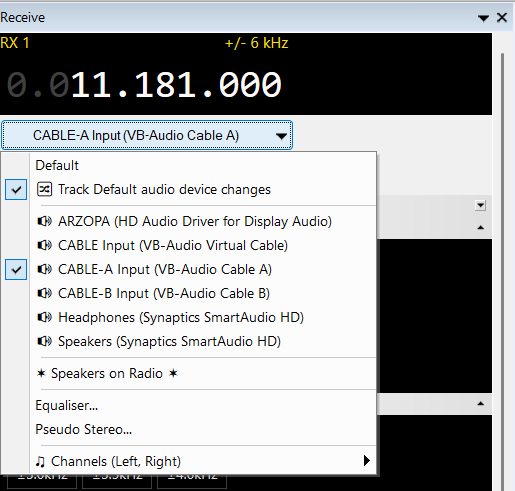
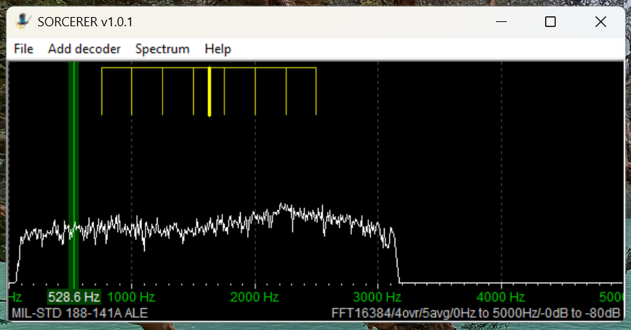
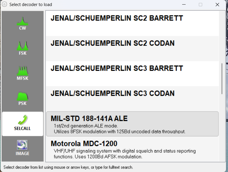
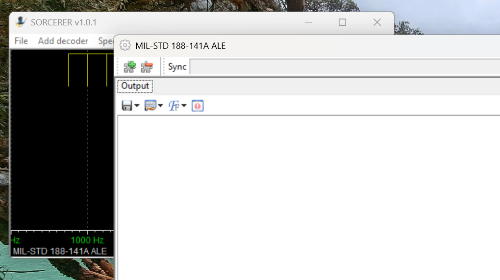
In the first two parts [Part 1 and Part 2] we looked at software used to decode ALE signals. Now let’s look at the stations and countries waiting to be logged.
If you’ve read the first two parts of this series then you know that there is no listening involved in ALE DXing. I know some traditionalists who would claim it’s not real DXing if you aren’t sitting next to the radio listening to a speaker or headphones. To me, DXing is having fun by logging new and interesting stuff. With ALE, the fun comes from researching the callsigns and frequencies to figure out what was logged. Every DX session produces numerous puzzles.
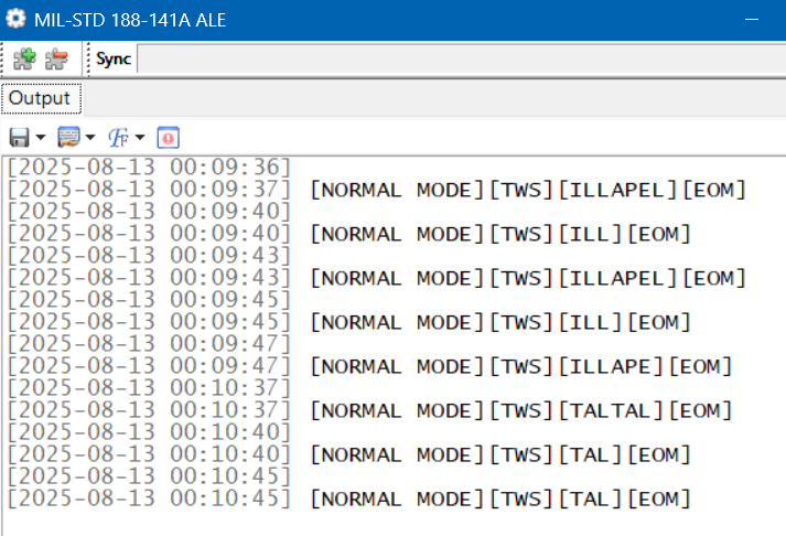
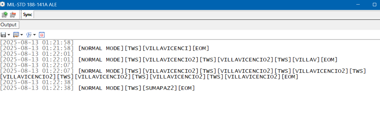
Identifying ALE stations may not sound hard. After all, one of the best things about monitoring ALE is that the stations are constantly identifying themselves. What could be easier? Unfortunately, it’s not always that easy to match up the callsign with what organization is behind it. Obvious location identifiers like ILLAPEL and VILLAVICENCIO2 are the exception, not the rule.
Around a third of the callsigns I decode stay complete mysteries as to who is behind them and where they are from. For about another third, the organization may be known (and, by extension, the country), but not the transmitter site. Only about a third of my ALE catches can be pinpointed exactly on a map as to where they came from. I wish it were more than that, but that doesn’t mean I haven’t logged some really interesting and unusual places.
Actually, it is surprising that I can pinpoint as many as I do. After all, every ALE network I’m aware of belongs to a government agency, a military, or some other government-affiliated organization. Bureaucracies like those are typically very careful about how they share information even when there is absolutely no security risk involved. Nevertheless, the utility DX community has gathered some excellent information over the years. While some of it is researched from public sources, I understand that some of it comes from inside sources that certain DXers have with people who install the networks. I don’t ask questions about where the information comes from and I’m glad to have the references and lists, which you can find in the links below.
Join the UDXF
The best source of ALE information is the Utility DXers Forum. The UDXF website has a lot of great utility resources that anyone can download. The best information, however, is the members’ loggings. To see those, you have to join the mailing list, where you can see member logs reported in the daily messages. But what you want to do is download the log compilations from the Files section (at Groups.io). Those go all the way back to the UDXF’s founding twenty years ago.
The first zip file is a compilation of all the logs from 2006 to 2019. After that, the logs are compiled into files for each year from 2020 to 2025. Download all of these and unzip them into a single folder. And periodically check back for newer files. At the beginning of each month, there will be a compilation for the previous month. Those will be compiled into a single file for 2026 at the beginning of next year. Finally, you need a way to search within the contents of an entire folder of files. A good text editor, such as Notepad++ for Windows, will do the job.
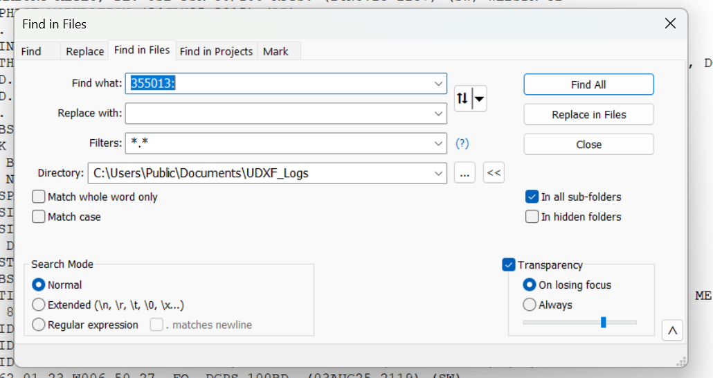
So let’s say I have a logging with the ID of 355013 on 8092 kHz. That really doesn’t tell me a thing about who could be behind the signal. Lots of organizations use six-digit strings as identifiers. I open up the Find in Files feature in Notepad++ and point it at the folder of UDXF logs. Now I type in the ID followed by a colon. Why a colon? Because in the UDXF logs, IDs are followed by a colon. By including the colon in my search term, I can eliminate any other random places that the same string of characters might be. (That’s more important when searching for shorter ID strings, such as three-digit numbers.)
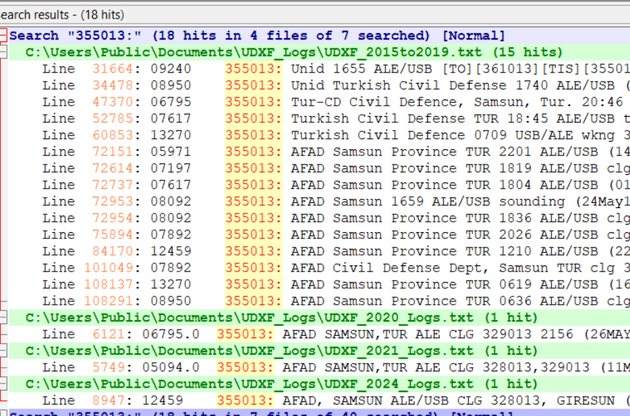
I click Find All and get back a listing of every line in those logs that contains my search string. I can click on any line to open that file at that point. In the frequency column here, I see two hits for this ID on 8092 kHz. I think I can be certain that this is the Turkish Civil Defense station in Samsun province.
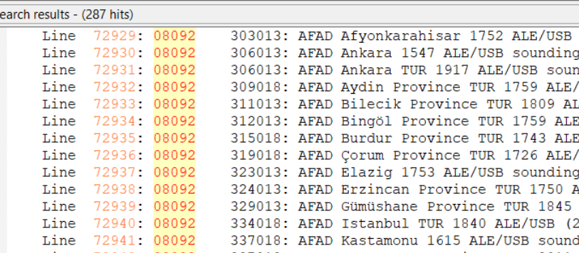
But what if I got these same results, but without any reports on 8092 kHz? That wouldn’t prove that I had logged Samsun even though the six-digit ID is a match on other frequencies. There are other organizations that also use six-digit numbers as IDs, such as UN Peacekeepers in several African countries. What I would do then is run a search for the frequency of 08092 (no colon) to see what other stations have been reported there. That turns out to be an important frequency in the AFAD network, so I could still safely assume that I had logged Samsun.
If the identifier doesn’t show up in the UDXF logs then there are some other resources (listed below) that can be checked. Sometimes the UDXF has complete network lists that include stations not yet reported in the logs. Another thing to do is look to see just what has been reported on that frequency. If there are lots of logs from a particular organization and the IDs follow the same pattern as the one you logged (e.g., six digits beginning with a ‘3’), then you likely got an unknown station in the same network.
If I get this far and still have no idea who is behind the station, then I have two options. I can delete the log and forget about it. Or I can put it in a ‘check later’ list, which I go through every year or so. I’ve identified a number of stations that way, especially from new networks. To be honest, which one I choose to do depends on how I feel that day!
Now let’s take a look at some of the places that stations can be logged from.
North America
The US government heavily uses ALE and there is no question that you will log more stations from the USA than from any other country.
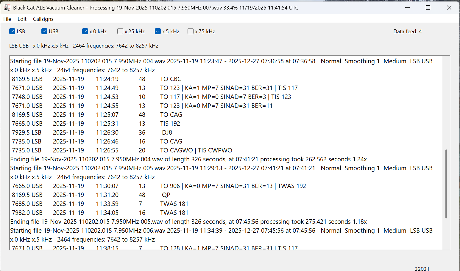
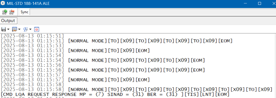
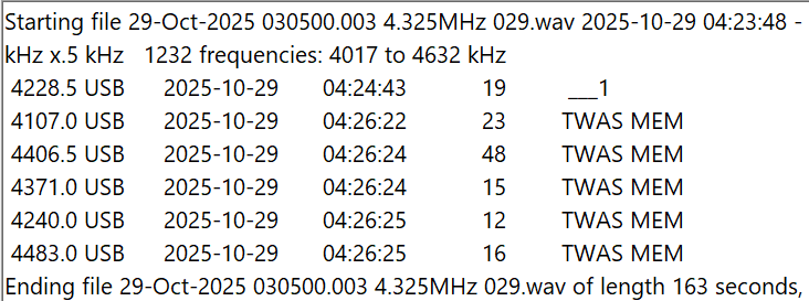
The most widely used set of frequencies by the US government includes 7527, 8912, 10242, 11494, 12222, and 15867 kHz. These frequencies are shared by several organizations, including the US Coast Guard, the FBI, the DEA (Drug Enforcement Agency), and the Customs and Border Patrol. The USCG is an especially heavy user, and it’s easy to log not only USCG bases but also USCG cutters at sea, as well as USCG aircraft. Another heavy user of these frequencies is the COTHEN network, or Cellular Over-The-Horizon Enforcement Network. This is a network of various law enforcement agencies and includes stations in some unusual places such as Limestone, Florida, and Lovelock, Nevada. Here is a string of Black Cat loggings on five different frequencies by MEM, the COTHEN station in Senatobia, Mississippi.
 Another large US government ALE network is run by FEMA (Federal Emergency Management Agency), which operates stations at each of its ten regional offices. The callsigns include the region number, e.g. FC4FEM1 from the region four office in Thomasville, Georgia. If you are in North America, it won’t take long to log all ten regions. Much rarer are the stations in individual state offices, such as SD8FEM in South Dakota and TN4FEM in Tennessee.
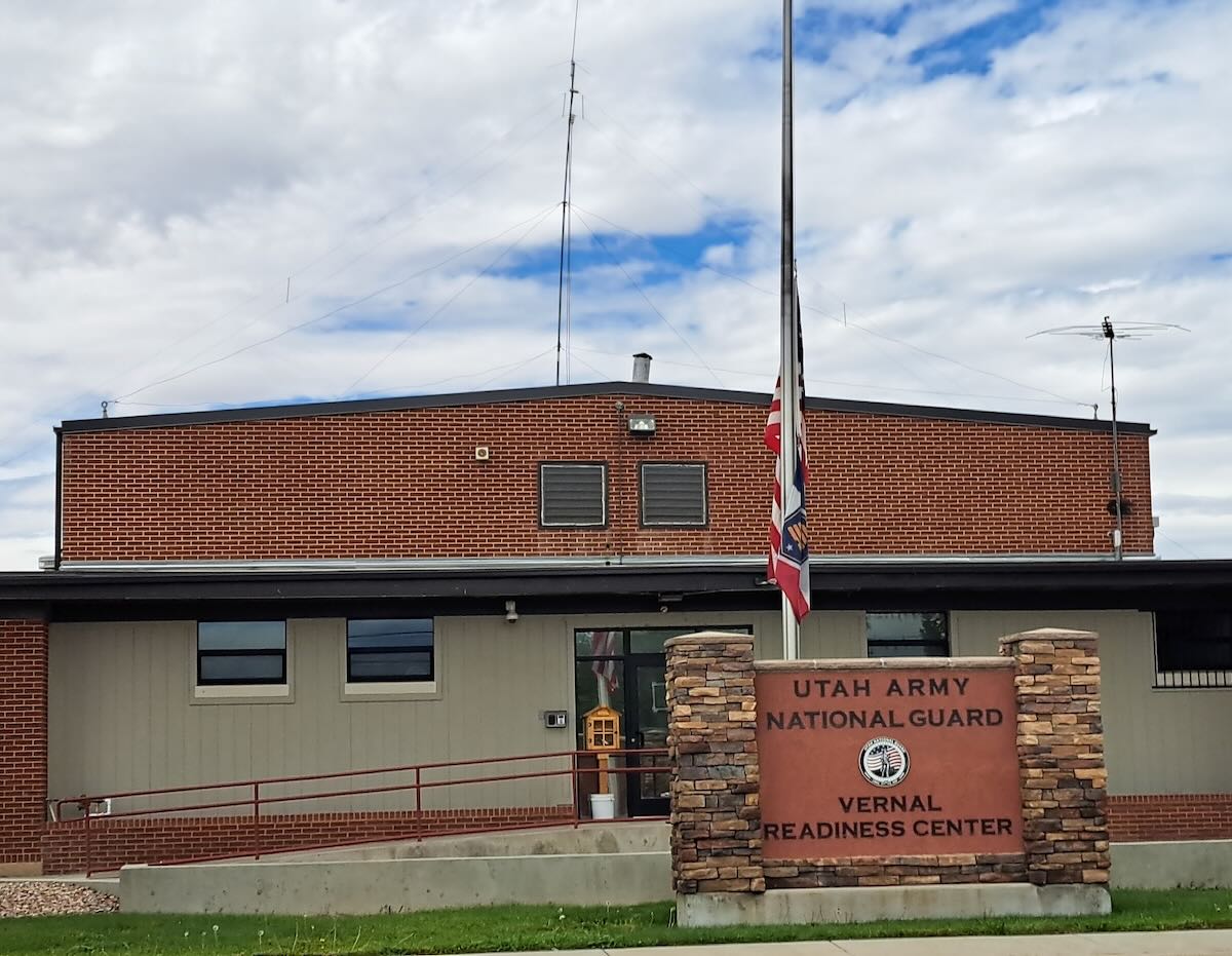
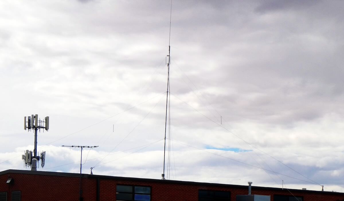
Some state National Guard units also operate on ALE, but by far the most active are the Wyoming and Utah National Guards. These can be logged on several frequencies, including 7805, 7932, and 8065. The Wyoming stations mostly identify by the full town name, e.g. LARAMIE or GILLETTE, while the Utah stations use the first three letters of the local base, e.g. AME for American Fork or TOO for Toole. In September, I passed through Vernal, Utah, and took these pictures of the Vernal National Guard center and the HF antennas on the roof.
Finally, there are several regional government and quasi-government organizations that can be logged. The most active network is probably the Bonneville Power Administration in the Pacific Northwest. It operates a handful of stations with calls including 1121BPA and 1351BPA. Unfortunately, there is no information as to where the individual stations are located.
US government ALE transmissions are not confined to the continental USA. As noted in part one of this series, the US Air Force operates from bases around the world. The US Coast Guard operates from Puerto Rico, Guam, Alaska, and Hawaii. The DEA has a station in Nassau, Bahamas. Finally, the US State Department operates from many consulates and embassies around the world.
The Canadian military has a few ALE stations on the air. Aside from that, to my knowledge, there is no ALE activity from Canada, Mexico, or any of the countries in Central America and the Caribbean, except for that done by the US government.
South America
The militaries of Brazil, Colombia, and Venezuela all operate ALE networks. The Brazilians seem to be particularly active. The police networks of Chile and Colombia, as mentioned in part one, are the most interesting as they identify with the station location. However, logging the Chileans in the northern hemisphere will require good conditions. I’ve only managed to get a few when DXing in the USA, although I have logged several more while DXing in South America.
Africa
Algeria is the heaviest user of ALE from Africa. The Algerian Air Force and Army operate from bases throughout this huge country, and in many cases, the exact locations of the stations are known. One of my favorite ALE logs is CM6 from Tamanrasset in the heart of the Sahara in southern Algeria. Sonatrach, the Algerian national oil company, also has a huge network of stations using four-digit numbers as identifiers. Unfortunately, there is no information as to the exact location of any of those stations.
Morocco, Mauritania, and Tunisia are three other countries with large ALE networks operated by their militaries and/or national police. Finally, United Nations Peacekeepers operate from several countries, including Mali, the Central African Republic, and South Sudan.
Europe and the Middle East
The United States may have the most ALE stations, but without a doubt, the most active ALE callsign is XSS from Forest Moor, England. Operated by the British military, this station pops up on dozens of frequencies throughout the shortwave spectrum. The previously mentioned Turkish AFAD operates what is probably the largest ALE network in this region. Another large network is Italy’s Guardia di Finanza, a sort of combination coast guard and tax enforcement agency. It’s hard to receive in North America, but I did once get one of their patrol boats. ALE is used by the militaries and border patrols of several other countries in this region. My best ALE catch from Europe is getting the Polish UN Peacekeepers in Kosovo. That’s my only logging of any type in that small country.
Asia and Pacific
Australian state police run an ALE network with 10505 kHz being a favorite frequency. To my knowledge, there is no other significant ALE activity in the region aside from that of various US government organizations.
That’s just a general overview of the major users of ALE, but there is a lot more to be logged that I didn’t mention. Unlike a lot of things on HF, the use of ALE is expanding, not contracting. For example, the Colombian police network didn’t even exist two years ago. So, give ALE monitoring a shot. I think you’ll find it to be one more way to make the DX hobby challenging and fun. I do.
Links
- The Utility DXers Forum website: https://www.udxf.nl/
- The Utility DXers Forum mailing list at groups.io: https://groups.io/g/UDXF
- A listing of networks and frequencies but not callsigns: https://ominous-valve.com/ale-list.txt