What’s in the Box?
Itemized by Bob Colegrove
Not one to throw anything away, I tend to save ‘the box it came in’ for many new purchases. The other day I decided to organize all my radio boxes. Besides the radios themselves, they usually contain a selection of “goodies,” which can include, cases, power adapters, USB cables, batteries, earbuds, antennas, manuals, and so forth.
I generally do not use much that is included in the box. Over time, however, some of the paraphernalia has gotten scattered around, and my recent effort was intended to corral and sort the accessories. My experience is itemized below.
Cases
The cases are invariably the largest accessories in the box. These are sometimes firm, faux-leather enclosures with a zipper around the edges. I prefer the soft, pliable pouches which seem to function more easily and take up less space.
The Sony ICF-2010 and -2001D did not include cases. To give the radio some protection during travel and storage, I fabricated a ‘sock’ out of an old bath towel and some hot glue. The so-covered radio was then inserted into a travel bag along with earphones and anything else I needed. This worked very well over the years; so well that I extended the concept for some of my smaller radios, which came with cases.

Homemade socks for a PL-880 and ICF-2010 could even be color-coordinated with the rest of your gear.
Power Adapters and Batteries
The following is not intended as the definitive treatise on power adapters and batteries. Enough guidance has been provided by others. The takeaway here is that, if you ever refer to the radio’s manual, this is the occasion to do so. Ensure you know how your radio was designed and the proper way to power it.
In my collection of portable radios there are several combinations of power adapters and batteries.
- Some radios came with power adapters and others didn’t.
- Some radios came with batteries and others didn’t.
- Some just came with USB charging cords.
- Some were intended for both chargeable and nonchargeable batteries. Others were intended only for alkaline, nonchargeable batteries, in which case the power adapter disconnects the battery from the circuit and is only used to power the radio.
An adapter might be used to power the radio, recharge batteries, or both. It’s hard to believe in these days of switching power adapters that an adapter could ever be used to listen to AM radio, but that was the case with the Sony ICF-2010/2001D and Grundig Satellit 800. These radios came with a more costly transformer adapter which produced very little discernable noise. Manufactured in pre-rechargeable alkaline days; however, the adapter did not provide a battery charge function. Over the years, I have mostly used these radios in-house. They tend to be D-battery-hungry, and so they are usually powered via the adapters.
When Sony got around to producing the ICF-SW7600GR, they took a different approach. They simply figured it was a small, portable radio, and would mainly be used with batteries. So, there is a power port for an optional 6-volt adapter, but no included adapter.
The OEM batteries aren’t always the best, so I have an extra supply of rechargeable NiMH and lithium batteries which I cycle through my radios, and the originals are simply included in the rotation. The NiMH batteries that came with the Tecsun PL-600, -660, and -680 only had 1000 ma capacity and tended to self-discharge quickly after a year or two of use. However, they got you started.
I have always wondered about using NiMH batteries in radios intended only for alkaline batteries – mainly older ones. There is a 20-percent reduction in voltage. How does this affect the performance of the radio? I suppose this can only be answered on a case-by-case basis. As an example, I have used NiMH batteries in the Sony ICF-SW7600GR from the very beginning with no apparent degradation. However, on the XHDATA D-219 and D-220, the difference is quite noticeable. For some radios, the battery type is switchable, and one must be careful not to connect a power adapter to recharge alkaline batteries.
Earbuds
If you’re serious about radio, you have a good set of earbuds or headphones. I would venture to say the supplied earbuds for each of my radios are still in the box in their original wrapping. I don’t get along well with earbuds. They are hard to install in what apparently are my constricted ear canals and are always falling out. Several years ago I purchased a set of quality over-the-ear headphones. Not the most convenient for travel perhaps, but great for reproducing sound and mitigating outside noise. Grundig went so far as to include a set of over-the-ear headphones with the Satellit 800.
Antennas
Most new portables come with 20- to 25-ft long wire external antennas having 3.5-mm plugs for connection to the external antenna jack. Sometimes a plastic ‘clothespin’ is attached to the remote end of the wire for mounting. For convenience, some of these wires are contained in a tape-measure-style spool. These antennas are quite useful for the non-tinker and traveler, as they provide a means to extend the range, particularly on shortwave.
The C. Crane wire terminal antenna adapter, included with the Skywave SSB 2, is a boon to anyone without a soldering iron or otherwise not inclined to use one. Other manufacturers take note. A #2 Phillips screwdriver, and knife to strip the wire insulation are all you need for extensive antenna experimentation.

Source: C. Crane Skywave SSB 2 Instruction Manual, p. 30.
Sony packed not one, but two 3.5-mm external antenna plugs with each ICF-2010/2001D. The concept was the same as the C. Crane wire terminal antenna adapter. These had wire pigtails ending in screw terminals for an antenna and ground wire of your choice.

External antenna adapter (1 of 2) packed with the Sony ICF-2010 and -2001D
A caution here. The RF amplifier for LW, MW, and SW on the 2010 is an unprotected FET (Q303), which is notorious for failing due to electrostatic discharge from an external antenna. Early on, your author was twice bitten by this snake. There may be other radios that suffer from this vulnerability.
Straps
The strap is arguably the least useful accessory included with any portable radio. The Sony ICF-2010/2001D came with a very attractive blue over-the-shoulder web strap, which has become something of an “item” among collectors. Mine have been bound up in their original wrapping and stored away for 40-plus years, and might yield the cost of a new portable radio should I ever decide to auction them on the Internet. I have never used them on either of my 2010s simply because I can envision the priceless radio dangling pendulously at the end of the strap waiting to meet disaster through contact with an immovable door jam.

The same goes for smaller radios which almost always include an obligatory wrist strap. Perhaps these should not be classified as accessories, as they are permanently attached to the radio. I avoid using them for the same reason as sited for the 2010s. Besides, they just get in the way. These straps are usually anchored inside the case, but I can’t bear to cut them off; so, I have just lived with them. In the few cases where I have opened the case, I have omitted reinstalling them. Instead of having a strap, how about a collapsible “lunchbox” handle? I can even envision one of these being developed into a dual-purpose handle/antenna.
Manuals
Don’t forget the manual. We’ve gotten away from manuals. People don’t use them, and they are a manufacturing expense. Besides, you can find your answer on the Internet.

As a retired technical writer, however, I have a strong respect for a well-crafted technical manual. Besides actually using them, I unconsciously evaluate them. Unfortunately, most are written as an afterthought – an attempt to forestall customer enquiries. “Read the manual.” The problem is compounded by radios intended for a worldwide market, wherein the manuals are authored by writers who labor under the handicap of having English, French, Spanish, German, etc. as a second language.
There are also situations where the printing is too small or the fanfolds too inconvenient. My standard practice is to download an electronic copy of each manual, print it out in 8 ½” × 11” format, and put it in a comb or 3-ring binder. This is easier on aging eyes, and more suitable for adding my own notes.
…and so forth
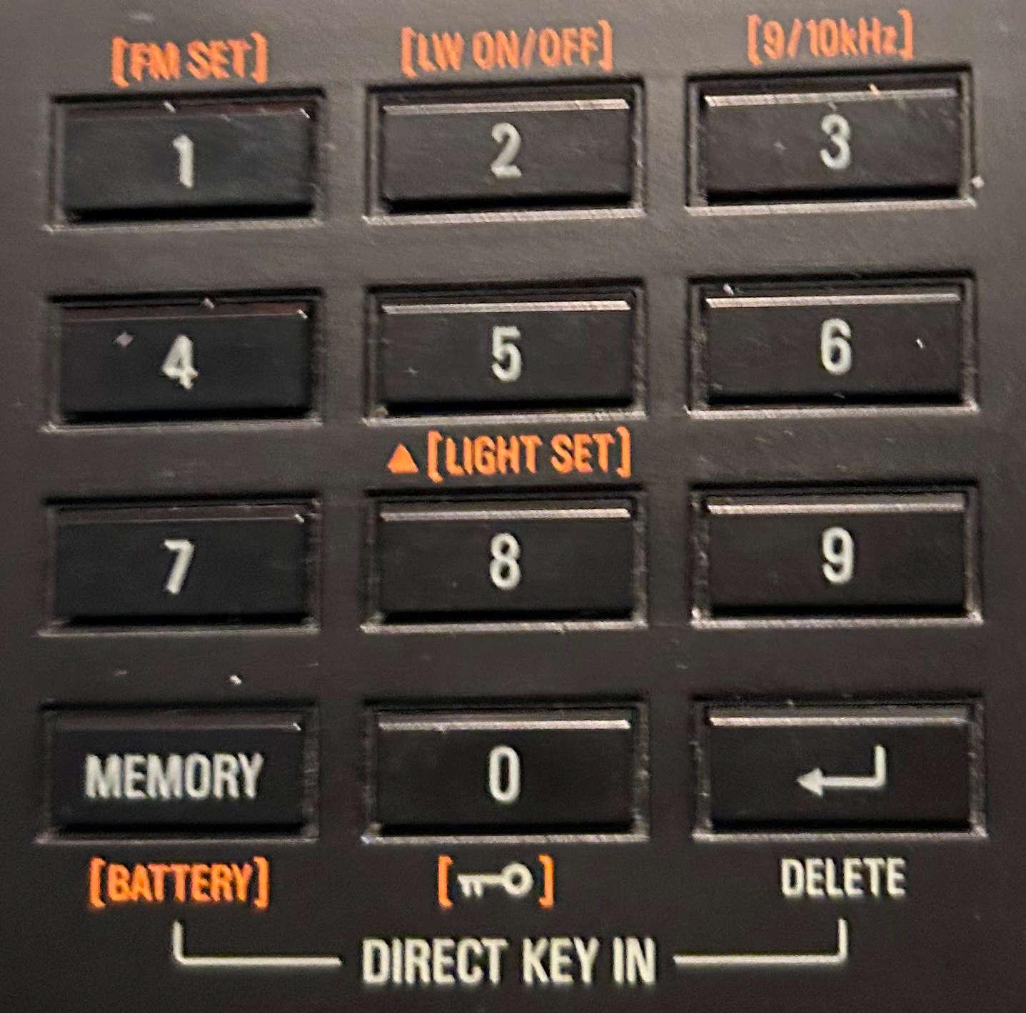
Besides the common accessories described above, some unique items have been included over the years. For example, Tecsun has packaged very nice 20-inch by 30-inch charts with some models. One side contains a world map showing amateur call areas. The other side is an enlargement of the radio with each button or control function described.

 Going back a few years, Sony included a slick publication called the Wave Handbook with some of their radios. These had convenient station vs. time charts for world band radio. The charts were like those published in frequency vs. time format in Passport to Worldband Radio. The booklets were published in several editions over the years, but obviously, these were time sensitive and became outdated rather quickly. Still, they could pique the interest of folks new to SWLing.

Packaging
Finally, there is the box the radio came in and any accompanying wrapping. The packrat DNA in me usually demands that I keep all this. It can speed up the sale or otherwise increase the value of the radio, if you ever decide to sell it.
Which radio accessories do you use?
Would you like an option to buy the radio without any accessories?