 Many thanks to SWLing Post contributor, Nick Hall-Patch, for sharing the following guest post:
Using Carrier Sleuth to Find the Fine Details of DX
by Nick Hall-Patch
Introduction
Medium wave DXers are not all technical experts, but most of us understand that the amplitude modulated signals that we listen to are defined by a strong carrier frequency, surrounded on either side by a band of mirror image sideband frequencies, containing the audio information in the broadcast.
Most DXers’ traditional experience of carriers has been in using the BFO of a receiver, using USB or LSB mode, and hearing the decreasing audio tone approaching “zero beat” of the receiver’s internal carrier compared with the DX’s carrier frequency as one tuned past it. This was often used as a way of detecting that a signal was on the channel, but otherwise wasn’t strong enough to deliver audio. Subaudible heterodynes, regular pulsations imposed on the received audio from a DX station, could indicate that there was a second station hiding there, with a slightly different carrier frequency, And, complex pulsations, or even outright low-pitched tones could indicate three or more stations potentially available on a single channel.
With the advent of software defined radio (SDR) within the last 10 years or so, the DXer has also been able to see a graphical representation of the frequency spectrum of the carrier and its associated sidebands. (Figure 1) Note that the carrier usually remains stable in amplitude and frequency, unless there are variations introduced by propagation, but that the sidebands are extremely variable.

Figure 1
Figure 2
In addition, by looking at a finer resolution of the SDR’s waterfall display, one might see additional carriers on a channel that are producing heterodynes (audible or sub-audible) in the received audio (Figure 2). Generally speaking, a DX signal with a stronger carrier will be more likely to produce readable audio, although there are exceptions to that rule.
Initially, DXers wanted to discover the exact frequency of their DX, accurate to the nearest Hertz. Although only a small group of enthusiasts were interested, they have produced a number of IRCA Reprints (https://www.ircaonline.org and click the “Free IRCA Reprints” button) over the years under the topic of “precision frequency measurement” (e.g. T-005, T-027, T-031, T-079, T-090) describing their use of some reasonably sophisticated equipment for the day, such as frequency counters.
So, why would this information be at all important? In effect, the knowledge of the exact frequency of a carrier was used to provide a fingerprint for a specific radio station. Usually, this detail was used by DXers who were trying to track down new DX, and wanted to determine whether a noisy signal was actually something that had been heard before, so would not waste any more time with it. The process of finding this exact frequency has since been made much easier by being able to view the carrier graphically in SDR software, assuming that the SDR has been calibrated before being used to listen to and record the DX. Playing back the recorded files will also contain the details of the exact frequency observed at the time of recording. And, because the exact frequency of DX has become much easier to determine using SDRs, more and more DXers seem to be using this technique.
At present, Jaguar software for Perseus is the one being used by many to determine frequency resolution down to 0.1Hz, both in receiving and in playback. But, if you have recorded SDR files from hardware other than Perseus, it is possible to get that resolution also, using software called Carrier Sleuth, from Black Cat Systems, available for both Mac and Windows, at a cost of US$20.
This software will presently take as input, sets of RF I/Q files generated by SpectraVue, SdrDx, Perseus (which includes files recorded by Jaguar), Studio One / SDRUno, Elad, SDR Console, and HDSDR. It then outputs a single file with a .fft extension, that provides the user with a set of waterfalls, similar to those displayed by SDR programs. The user decides ahead of time which frequency or set of frequencies (including all 9kHz or all 10kHz channels) will be output, and these will be displayed as individual waterfalls. one for each chosen frequency. These waterfalls can be stepped through from low frequency to high frequency, or chosen individually from a drop down menu.
Let’s start by looking at a couple of output waterfalls and work out what can be done with them, then step back to find out how to generate them, and what other data is available from them. Finally, we’ll do a quick comparison with two other programs that can produce similar output, and discuss the limitations in all three programs.
Example outputs from Carrier Sleuth
An example showing the original intent of Carrier Sleuth, determining precise carrier frequencies, is shown in Figure 3, a waterfall from 1287kHz on the morning of 28 November 2020. At 1524UT, a woman mentions “HBC” and “Hokkaido” in the original recording, so, it’s JOHR, Sapporo. Although there are a number of vertical lines representing carriers in this graphic, only one has a strong coloration, indicating at least 25dB more strength than any other carrier at the time of the ID, and about 50dB more than the background level. The absolute values of time, signal strength, and carrier frequency precise to 0.1Hz, can be found by mousing over the desired point in the waterfall and then reading the numbers in the upper right corner of the display, (encircled in Figure 3). In this case, the receiver’s reference oscillator had been locked to an accurate 10MHz clock, disciplined by GPS, so the frequency indicated in the software is not just precise, but should also be accurate. Similar accuracy could be obtainable by the traditional method of calibrating the SDR to WWV on 10 or 15MHz.
Carrier Sleuth indicates 1287.0002kHz, within 0.1Hz of that observed by a contributor to the MWoffsets list about 7 weeks earlier (https://www.mwlist.org/mwoffset.php?khz=1287). If you look closely, there is a slight wobble on the frequency, but the display is precise enough that it can indicate that, despite the wobble, JOHR does not wander away from that frequency of 1287.0002kHz.

Figure 3
But let’s face it, tracking carriers to such accuracy is a specialist interest (though admittedly, the medium wave DXing hobby is full of specialist interests, and this one is becoming more mainstream, at least among Jaguar users). However, if I played back a file from another morning, and found a strong carrier on a slightly different frequency from 1287.0002kHz, it might be an indication that some new Chinese DX was turning up, and that the recorded files would be worth a closer listen at that particular time.

Figure 4
In fact, I’ve found Carrier Sleuth to be useful in digging out long haul DX after it’s been recorded, as both trans-Arctic and trans-Pacific DX at my location in western Canada can be spotty at the best of times. This means spotty as in a “zero to zero in 60 seconds” sort of spotty, because a signal can literally fade up 10 or 15dB to a readable level in 20 seconds, perhaps with identifiable material, then disappear just as quickly. My best example so far this season was on 1593kHz, early in the UTC day of 16 November 2020, when a Romanian station on that channel paid a brief visit to my receiver in western Canada. An initial inkling of that showed up in a Carrier Sleuth waterfall, a blotch of dark red at 0358UT, and indicated by the yellow arrow in Figure 4; that caused me to go back to the recorded SDR files that had generated these traces.
The dark blotch indicates a 10dB rise and fall in signal strength including about 60 seconds of rough audio, which turned out to be the choral version of the Romanian national anthem (RCluj1593.wav). That one carrier and another one both started up at 0350UT, the listed sign-on time for Radio Cluj, which does indeed begin the broadcast day with that choral anthem. Which one of the Radio Cluj transmitters was heard is still an open question, due to the lack of carrier sleuths (computerized or otherwise) on the ground in Romania, but the more powerful one listed is a mere 15kw, so I will take either.
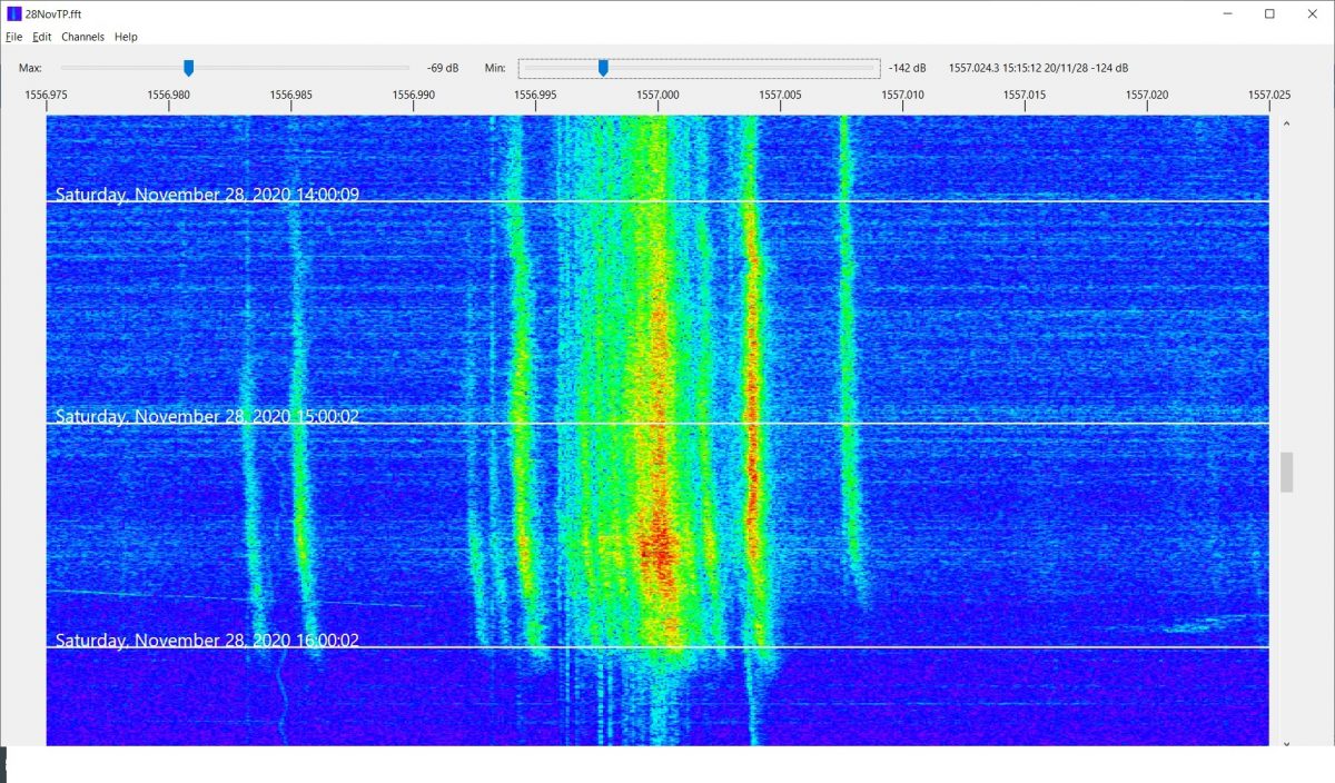
Finally, for those who have interest in radio propagation, the Carrier Sleuth displays can reveal some odd anomalies, for example, Figure 5 which displays both Radio Taiwan International (near 1557.000kHz on 28 November, but varies from day to day), and CNR2 (1557.004kHz) carriers as local sunrise at 1542UT approached in Victoria, BC.
Figure 5
The diffuseness of the carriers is striking, as is their tendency to shift higher in frequency at local sunrise. This doesn’t seem to be some strangeness in the original SDR recording, as there appear to be unaffected weak carriers on the channel. For comparison, Figure 3 shows the same recorded time and date, but on 1287kHz, and JOHR’s carrier is pretty stable, but there are others on that channel that show the shift higher in frequency around local sunrise. As one goes lower in frequency, these shifts became smaller and less common on each 9kHz channel, and disappear below about 1000kHz. On later mornings, however, the shifts could be found right down to the bottom of the MW band. Certainly, these observations are food for further thought.
Many of the parameters in Carrier Sleuth are adjustable by the user, for example, the sliders at the top of the screen can allow adjustment of the color palette to be more revealing of differences in signal strength. The passband shown is also easily changed, and in fact, setting the passband width to 400Hz, instead of my usual 50Hz , and creating another run of the program on 1557kHz, shows very clearly the sidebands of the “the Rumbler”, a possible jammer on the channel (Figure 6). Incidentally, a lot of the traces around 1557.000kHz in Figure 5 may well be part of “the Rumbler” signal as well, as filtering of the audio doesn’t seem to improve readability on the channel.
Although the examples here are taken from DXing overseas signals from western Canada, there is no reason why similar techniques may not be applied to domestic DXing, particularly during the daytime, when signals can be weak, but can fade up unpredictable for brief periods.
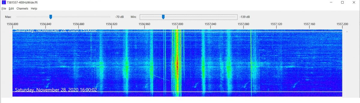
Figure 6
How to create these waterfall displays in Carrier Sleuth?
So, how can you get these displays for yourself? A “try before you buy” version of the program is available at http://blackcatsystems.com/software/medium_wave_carrier_display_app.html and both the website and the program itself contain a quite detailed set of instructions. However, the 25 cent tour can be summarized this way:
You start with a group of supported SDR data files, previously recorded, and use “Open I/Q data files” in the File drop down menu. Figure 7 shows the window that will open to allow you to choose any number of the files from your stored SDR files, by clicking the Add Files button circled in red. Then choose one of the options inside the green circle in Figure 7. They are explained in more detail in the help write up; note that the “Custom Channel” can be specified to considerably more precision than just integer kHz values, e.g. 1205.952 The rest of the settings you will probably adapt to your needs as you gain experience. Finally, set an output file name using the Set Output File button, and hit the “Process” button at the bottom of the window. There are a couple of colored bars in the upper right hand corner of the display that indicate progress, along with number of seconds left, although these are not always visible.
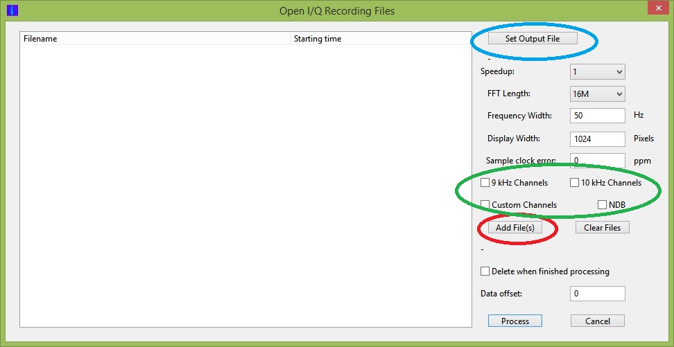
Figure 7
The generation of these waterfalls takes time. A computer with a faster CPU and more memory will speed things up. There is, however, an important limitation of the program. It is specified for 32-bit systems, and although it will run with no problem on 64-bit systems, individual input I/Q files are therefore restricted to 2GB or less. Many SDR users now choose to create larger files than this, and Carrier Sleuth will not handle them. Another possible limitation can occur when processing 32M FFTs, which are useful for delivering very fine frequency resolution of the carriers displayed. The program really requires in excess of 4GB of memory to handle the computation needed to deliver this fine a scale. Unfortunately, both the 2GB file size limitation and insufficient memory limitation deliver generic error messages, followed by program termination, which leaves the inexperienced user none the wiser about the true problem.
This might be a good place for a word about FFT size and Resolution Bandwidth (RBW). The FFT is a mathematical computation that takes as its input the samples of digital data that an SDR generates (or those samples that have been saved in recorded files), and generates a set of “bins”, which are individual numbers representing signal strength at a defined number of consecutive frequencies spaced across the full bandwidth being monitored by the SDR. You could think of these bins as a series of tiny consecutive RF filters, spread across the band, each delivering its own signal strength. As we are trying to look at fine scale differences in frequency when using a program like Carrier Sleuth, it is important that these little “RF filters”, or bins, each have a very narrow bandwidth. This value is called “Resolution Band Width” (RBW), and preferably should be a fraction of a Hertz to get displays such as those shown in Figures 3 through 5.
The “FFT Length” is the number of bins that the FFT display contains, and is equal to the number of I/Q samples (either from the SDR or recorded file) that are used for the input to its computation. The relationship between FFT Length, the bandwidth of the SDR or of the original recorded I/Q file, and the RBW is fairly simple:
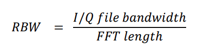
Because the MW DXer is usually looking at data with 1MHz or more bandwidth, this equation tells us that to get a smaller than 1Hz RBW, we will need to have an FFT length of well over one million bins, so it would be wise to use an FFT length at least 8M(illion). If you are looking at a recorded file that is from an SDR using a lower bandwidth, then a lower FFT length will do the job to get a smaller RBW.
A downside of using a long FFT length is that the time resolution of the FFT becomes poorer, resulting in a display in Carrier Sleuth that will appear to be compressed from top to bottom compared with what was seen when recording the SDR file, and with correspondingly less response to fast changes in signal strength. However, using a 16M FFT Length on a recording of the MW band results in a time resolution of about 12 seconds, so it should not be a deal breaker for most.
Producing signal strength plots
A further specialist activity for some DXers is recording signal strength on specific channels, and then displaying the progress of signal strength versus time, often to indicate when openings have occurred in the past (say, at transmitter sunset), and perhaps allowing one to predict such openings in the future. But, the world has come a long way from the noting down of S-meter readings at regular time intervals, both in deriving signal strength and in plotting the results. Read on for an example.

Figure 8
Carrier Sleuth recently added the capability of creating files containing signal strength versus time for specified frequencies, and, depending on the size of RBW, to deliver that signal strength as observed in a passband as narrow as 0.05Hz, or as wide as 10Hz. The program extracts the signal strength information from one of the FFT files that it has already generated from a selection of SDR I/Q files. In Figure 5, two stations’ signals, from Radio Taiwan International, and from CNR2, were featured in the display. With roughly 4Hz difference between the two signals, it is easily possible with Carrier Sleuth to derive signal strength from each one, specifying a bandwidth of, say 1.2Hz, to account for the propagation induced drifts and smearing of the carriers, not to mention any drift in either the receiver or transmitter.
The program creates a .csv file (text with comma delimiters) of signal strength versus time for all the frequencies chosen from an individual FFT file, but does not plot them. There are several programs that can create plots from CSV files For example, an Excel plot generated from Figure 5 is in Figure 8, showing peaks in those signals that occurred both before and after local sunrise at 15:42UTC. Note that the user is not restricted to the signals found on just one of the waterfalls that are found in the FFT file, but can pick and choose dozens of signals found anywhere in those waterfalls. (Note also that one can choose locations on any waterfall where there is no signal trace, in order to provide a “background level versus time” in the finished plots, if desired)
The process used to generate this CSV file involves searching through the FFT waterfalls for signal traces that are likely candidates for adding to such a file. On the first candidate found, the user right clicks the mouse on the trace, at the exact frequency desired; this will bring up an editable window. The window will show the chosen frequency as well as any subsequent ones that will be chosen, then the overall selection is saved to a text file after editing, so that the user can move on to generating the CSV file.
That file is created by going to the File drop down menu, and choosing “Generate CSV File”, where the text file produced earlier can be chosen. Once that file is selected, the CSV file is immediately generated, and can then be manipulated separately as the user chooses.
Are there comparable programs?
Displaying waterfalls in SDR programs playing back their own files is nothing new, though not that many can do it at as fine a scale as Carrier Sleuth does, and most programs are not optimized to handle such a variety of input I/Q files.
One that does read a fair number of different kinds of SDR files is the SDR Console program; this includes Data File Analyser (64-bit only) which also can display carrier tracks to a high resolution, so let’s take a quick look at what Analyser does. If you are familiar with SDR Console, and are reasonably experienced with the way it handles your SDR or plays back files from your favored SDR software, then these online instructions https://www.sdr-radio.com/analyser will help you get started with Analyser
This program will input a group of SDR files, then display an equivalent to a single one of the waterfalls output by Carrier Sleuth, displaying the carrier traces in reverse order, with time running from bottom to top of the display. Figure 9 shows the equivalent of Carrier Sleuth’s display of the 1287kHz carrier traces shown in Figure 3. Analyser has a convenient sliding cross hair arrangement (shown in the yellow oval) to reveal time and frequency at any point in the display, but the actual signal power available at that point must be derived from the rough RGB scale along the left hand border. Analyser is apparently capable of about 0.02Hz resolution when reading from full bandwidth medium wave SDR files, but the default is to display exact frequency only to the nearest Hertz. The “Crosshairs” ribbon item has a drop down of “High-Resolution” which displays to the nearest milliHertz however, though that will be limited by the actual RBW of the generated display. The graphic display can be saved as a project after the initial generation of the signal traces, which allows the user to return to the display without having to generate it all over again, equivalent to opening one of Carrier Sleuth’s FFT files.
A useful facility in Analyser is the ability to click “Start” in the Playback segment of the ribbon above an Analyser display, then mouse over and click on a signal trace; this action will play back the audio for that channel in SDR Console, at that point in time.
It is possible to generate a signal strength plot of signal strength versus time for any individual frequency in the waterfall display, and to save that plot as a CSV file (“Signal History”). But, the signal strength is that found only in a +/- 0.5Hz passband around the chosen frequency, with no other possibilities. If you want to generate a plot for another frequency on the same waterfall, then you will need to run the process again, and if you want a plot for another frequency in the SDR files, then you need to generate another waterfall, which, depending on your computer’s capability, could take some time. On an i3 CPU-based netbook with 4GB of memory, it took 30 minutes to produce one frequency’s worth of traces from data files scanning three hours. On the same machine, Carrier Sleuth could deliver all 9kHz channels in 1hr20min from the 3 hours of files. However, it also took 1hr20min to play back just one channel in Carrier Sleuth, which is not so efficient. (further note: Nils Schiffhauer has developed a technique to speed up Data Analyser processing, by first using Console’s Data File Editor on full bandwidth MW recorded files; details will likely appear at https://dk8ok.org)
To conclude then, SDR Console’s Analyser will produce a display of a single channel faster than Carrier Sleuth will, and will play back the audio associated with that channel, while also having the capability to plot and record signal strength for a single given frequency within that display, but only on 64-bit computers. It can also handle SDR files larger than 2GB in size, and will run more quickly if a NVIDIA graphics card has been installed. Analyser is also strict about sequence of files. If there is the slightest gap between one file finishing, and the next file starting in time sequence, it regards that as a new set, that will need to be processed separately.
Where Carrier Sleuth is more useful is that once an FFT file has been generated, it is easy to quickly check multiple channels for interesting openings during the recorded time period. It can also provide very precise frequencies of carriers, and is able to generate a file of signal strengths versus time from multiple frequencies, including those frequencies that are separated by barely more than the RBW. For the MW band, that can be near 0.1Hz, often beyond the capability of transmitters to be that stable. See Figure 10, which shows signal strength traces from JOCB and HLQH both on 558kHz, and separated in frequency by 0.1Hz. At 1324UTC, JOCR dominates with men in Japanese, and at 1356UTC, the familiar woman in Korean dominates, indicating HLQH.
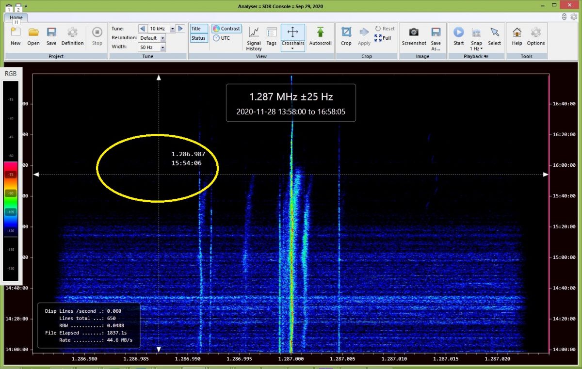
Figure 9
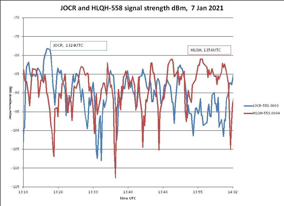
Figure 10
Incidentally, another program that seems to offer a similar functionality to Carrier Sleuth and SDR Console’s Analyser is, of course, Jaguar, which has made a point of displaying 0.1Hz readout resolution when using the Perseus SDR, and in playing back Perseus files, but…only Perseus. There is a capability called Hi-Res in Jaguar Pro that can be applied when playing back files; this also displays fine scale traces of frequency versus the passage of time. Steve VE6WZ, sent the example shown in Figure 11, zeroing in on his logging of DZAR-1026. As with Analyser, clicking on a certain point in the display plays back the audio at that time, but it is unclear at this point whether the display can be saved, or whether it is generated only for one individual channel, and then is lost.
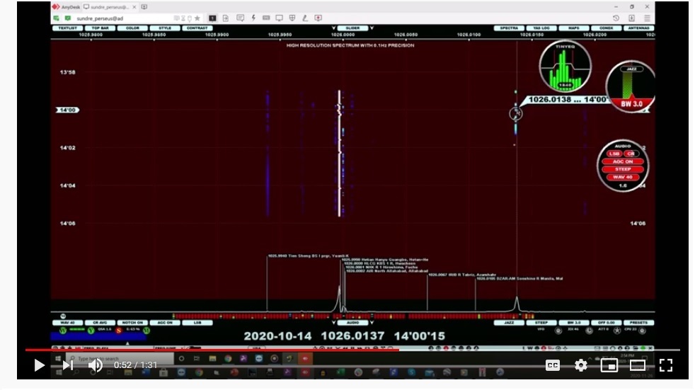
Figure 11
+ + + + + + + + + + + +
Availability
Carrier Sleuth http://blackcatsystems.com/software/medium_wave_carrier_display_app.html
Analyser (SDR Console) https://www.sdr-radio.com/download
Jaguar http://jaguars.kapsi.fi/download/ (these are the Lite versions; to unlock the Pro version, purchase is needed)
(this article first appeared in International Radio Club of America’s DX Monitor)
Many thanks, Nick. This is amazing. What a brilliant tool to find nuances of a DX signal. I can’t help but marvel at the applications we enthusiasts have available today. Thank you for sharing!

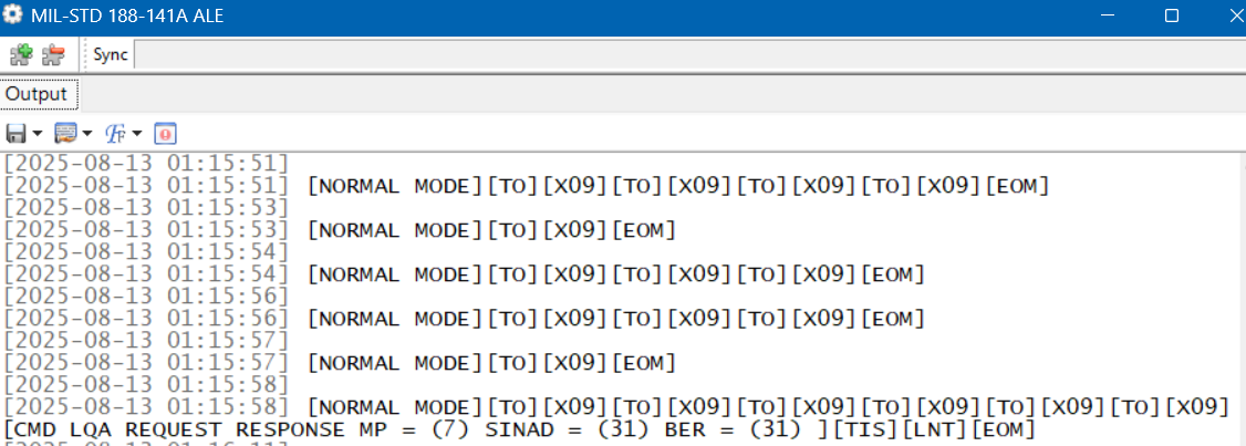
 A Beginner’s Guide to ALE: Part Three
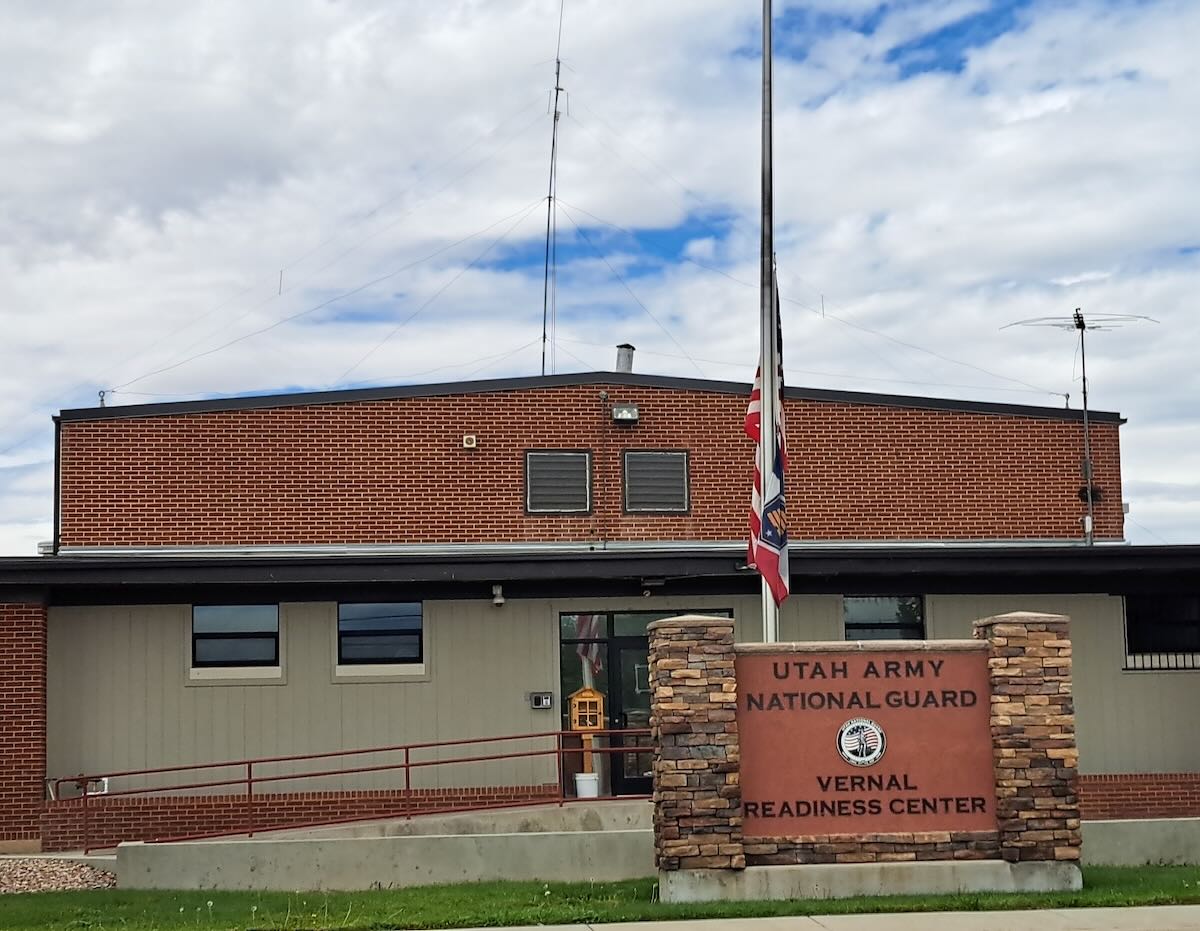
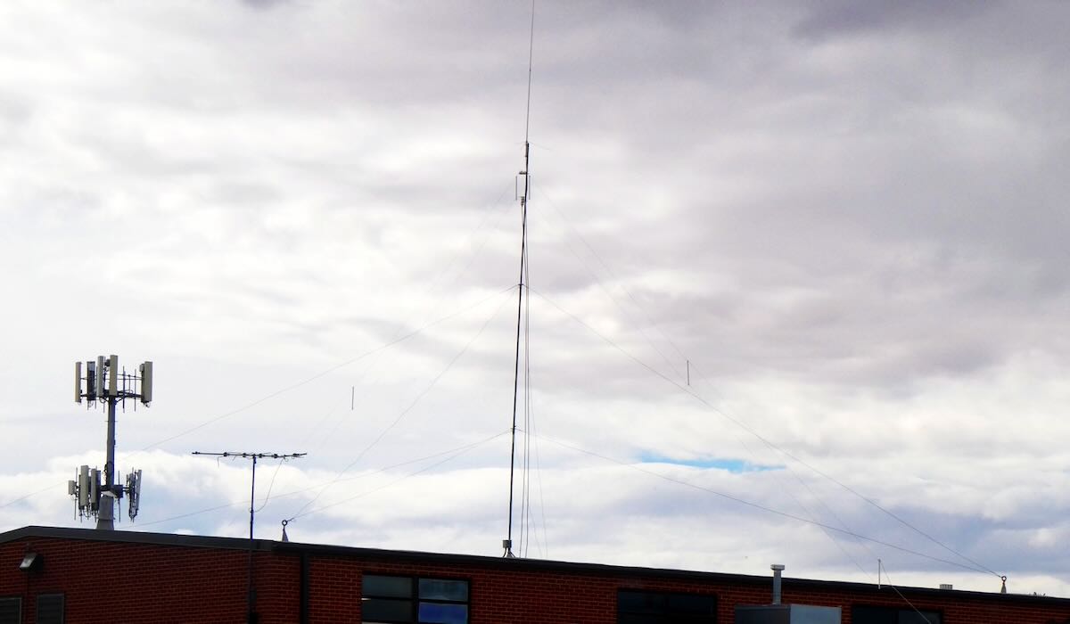
 Another large US government ALE network is run by FEMA (Federal Emergency Management Agency), which operates stations at each of its ten regional offices. The callsigns include the region number, e.g. FC4FEM1 from the region four office in Thomasville, Georgia. If you are in North America, it won’t take long to log all ten regions. Much rarer are the stations in individual state offices, such as SD8FEM in South Dakota and TN4FEM in Tennessee.