Many thanks to SWLing Post contributor, Dennis Dura, who shares the following video via YouTube:
Click here to view/listen via YouTube.
Wonderful recording. Thank you for the tip, Dennis!
Many thanks to SWLing Post contributor, Dennis Dura, who shares the following video via YouTube:
Click here to view/listen via YouTube.
Wonderful recording. Thank you for the tip, Dennis!

By Jock Elliott, KB2GOM
It was a reader, Mario Filippi, who set me on this path. He posted a comment that said, in part: “An interesting place to DX would be the segment between 1500 – 1590 kc’s where there are a number of news stations, one being federal news on 1500.”
Huh, I thought, federal news? I wonder if I can hear that. So I hooked up the MFJ 1886 Receive Loop Antenna to my Grundig Satellit 800 receiver and tuned to 1500. With the 800’s whip antenna, I heard mostly static; switching to the 50-foot indoor room loop, pretty much the same; same thing with the 1886 with the amplifier turned off. But turn the 1886’s amplifier on, and it was like getting slammed against the wall by the schoolyard bully: LISTEN TO ME! A big, fat, S9 signal, sounding like WGY 810 just a few miles from me. Wow, I thought, this loop can really pull out a signal.
A little research revealed, as nearly as I can tell, that Federal News 1500 is in Washington, DC, over 300 miles from me. Over the next few days I would occasionally check on Federal News 1500 using the 1886 loop, and typically it was loud and clear here in Troy, NY.
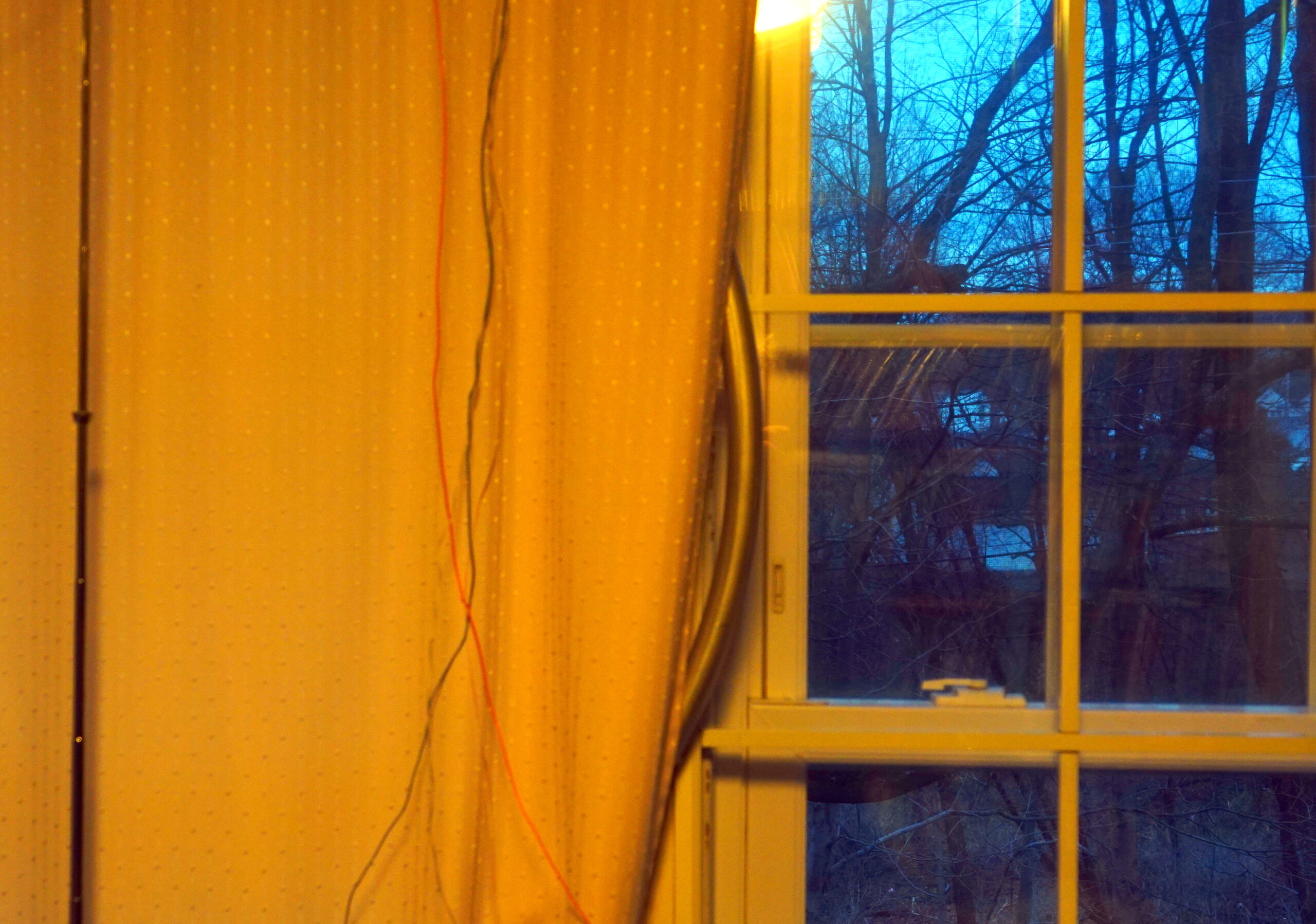
Hidden behind a curtain, the 3-foot aluminum loop of the MFJ 1886 works well for MW DXing.
Early this morning, Jan. 28, 2023, a thought crept into my brain: how many big, fat, MW signals could I detect with the combo of the Satellite 800 and the MFJ 1886 loop antenna? (Bear in mind that my 1886 rests flat against a window and is NOT rotatable in its current configuration.) Here’s the log, with station IDs when I could get them.
Time Frequency Station
1100Z 1520 WWKB Buffalo
1102Z 1530 Milwaukee? Sports, Australian open
1106Z 1540 CHIN Toronto, old time radio programs
1112Z 1560 religious music
1115Z 1660 orchestral music, Strauss waltzes
1118Z 540 middle eastern music
1121Z 660 WFAN, NYC
1124Z 700 WLW, Cincinnati
1127Z 710 WOR, the Voice of New York
1129Z 730 French language, Canada mentioned
1132Z 750 WSB, Atlanta
1134Z 770 WABC, NYC
1135Z 790 ortho doctor show
1138Z 860 French language, Canada mentioned
1140Z 880 WCBS, NYC
1142Z 1010 WINS, NYC
1144Z 1020 Talk
1146Z 1030 WBZ, Boston
1148Z 1050 WEPN, ESPN radio, New York
1149Z 1060 KYW, Philadelphia, PA
1153Z 1090 WBAL, Baltimore
1154Z 1110 WBT Charlotte, NC
Bottom line: it was immense fun, tuning around for “fat” MW stations in the early AM. Periodically I checked the other antennas as I traversed the band, but universally the MFJ 1886 was better at pulling them in.
Fat station DX? You bet! Try it; you’ll like it!
 Many thanks to SWLing Post contributor, Don Moore–noted author, traveler, and DXer–for the following guest post:
By Don Moore
When I was in college over forty years ago, seven of us had a small DX club in central Pennsylvania. A couple of times a year we would gather at the house of one of our parents for an all-night DX session. We shared tips and ideas, had fun, and always heard some new DX. Good DX can happen anywhere if conditions are right and most of mine over the past fifty years took place at wherever home happened to be at the time. But most of my best experiences and best memories of DXing were not made at home. They were made by getting together to DX with other hobbyists such as we did back in college.
Nowadays when I get together to DX with other hobbyists it’s to go on a DXpedition, which is nothing more than taking your receiver to a place where DXing will be better than at home because there’s less noise and you can erect better antennas. Simple DXpeditions can be done from cars. My old friend Dave Valko used to go on what he called micro-DXpeditions. He drove to a remote spot in the mountains not far from town, laid out a few hundred feet of wire, and then DXed from his car for a couple hours. He frequently did this around dawn and around sunset and got some great DX. I know several other DXers that do this today, either at countryside locations or in large parks.
I’ve done micro-DXpeditions a few times. It’s fun but it always lacks an important element: other DXers. For me, the best DXpeditions aren’t just about hearing interesting stuff (although that is very important). They are also about sharing the hobby with other interested friends. And the best way to do that is to go on a real DXpedition with them.
For three years in a row prior to the pandemic a group of eight of us had rented a lodge in rural central Ohio for an annual DXpedition. Covid shelved our plans for 2020 but by the summer of 2021 we were all looking forward to a fourth DXpedition in September. Then another wave of covid swept across the country and we canceled a few weeks before the event. Fortunately, the worst of those days are behind us and we finally had our fourth DXpedition the first week of October of this year. Unfortunately, only five of us could make it – Ralph Brandi, Mike Nikolich, Andy Robins, Mark Taylor and I.
For four nights our DXpedition home was the same place in western Pennsylvania that we had canceled at in 2021. The location was a rural house on the bluffs overlooking the Allegheny River near the old East Sandy railroad bridge (now a hiking trail). It’s always a gamble going to a new place chosen solely based on the AirBnB listing and other information found online. But this site had all the appearances of being a good place to DX from. The pictures and Google satellite view showed that there were trees around the house and large nearby open fields surrounded by woodland. The terrain was relatively flat when viewed on 3D satellite view. We would have plenty of space for a variety of antennas. Furthermore, it didn’t look to be a noisy location. The nearest neighbor was over a quarter mile to the south and because the house was the last one on the road that powerlines stopped at the driveway. I couldn’t have done much better if I had designed the location myself.
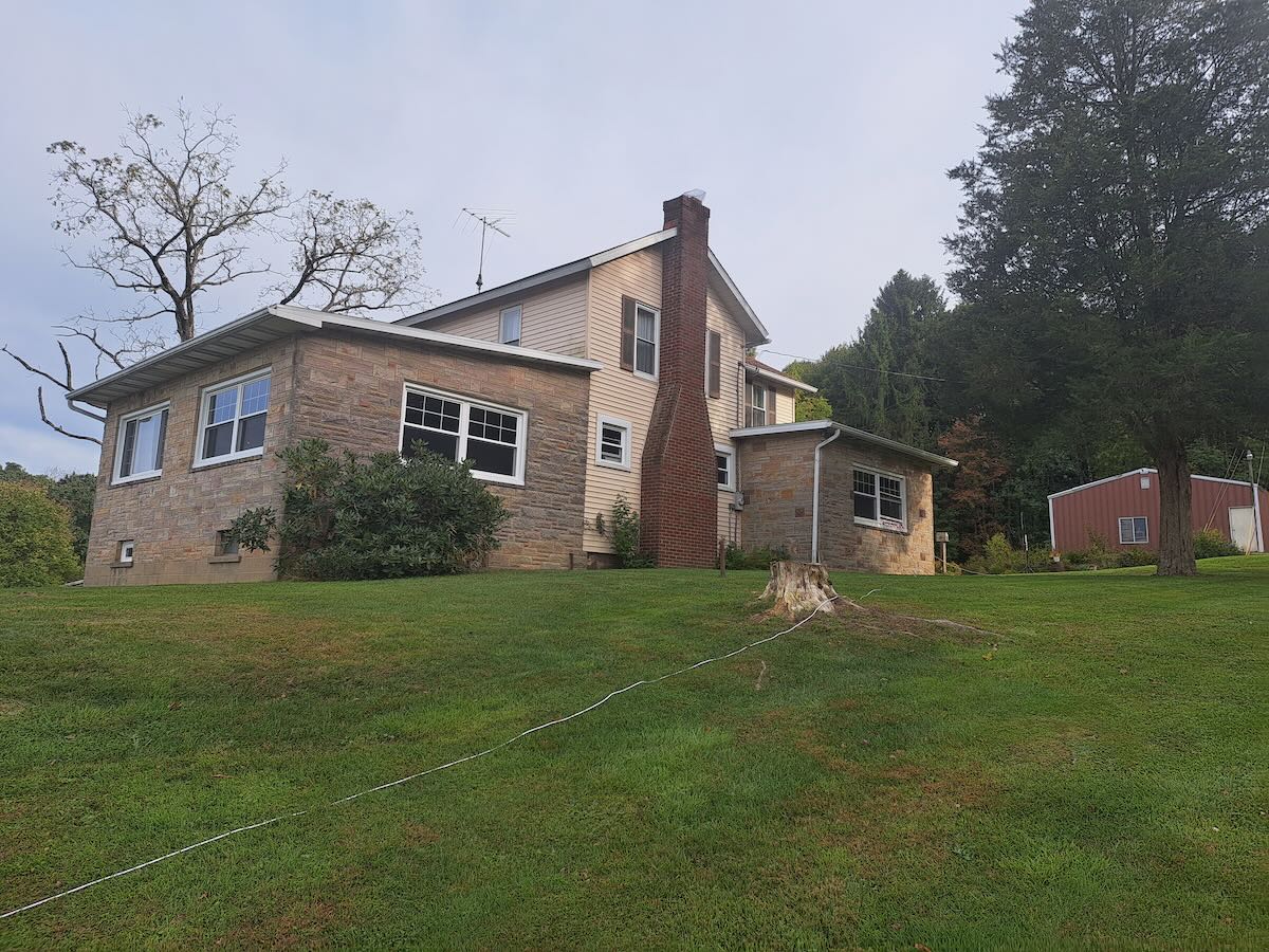
Our DXpedition home. Coordinates 41°19’23″N 79°46’08″W (Don Moore)
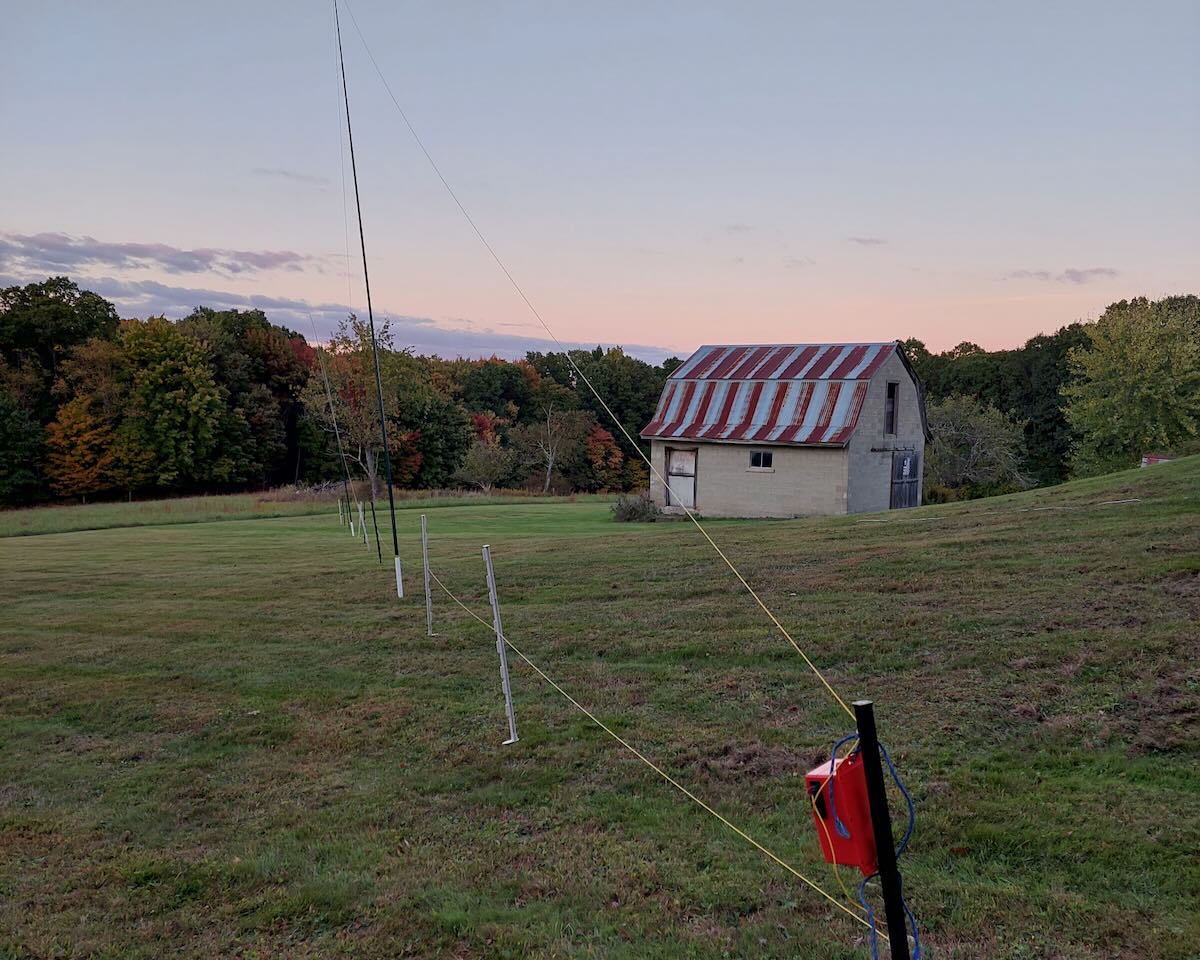
Good antennas are the most important part of any DXpedition and erecting them is usually the most time-consuming part of set-up. Still, you never really know what’s going to fit until you’re there. I arrived at 2 p.m. and Mark pulled in a few minutes later. We immediately walked the grounds and were pleased with what we saw. Ralph arrived while we were laying out the first antenna. Mike and Andy arrived later in the afternoon in time to help finish up.
Our DXpedition antenna farm consisted of two delta loops, a DKaz, and two BOGs. The delta loops used Wellbrook ALA-100LN units and are as I described a few years ago in my article on radio travel. These are easy to erect and are good all-around antennas for anything below 30 MegaHertz. The DKaz (instructions here) is a rather complex-to-build antenna designed for medium wave. Ralph uses one at home which he had taken down for the summer to make yard work easier. He brought the pieces and put it up by himself. The two BOGs (Beverage-on-the-ground) were a 300-meter wire to the northeast and a 220-meter wire to the north. Beverages are good for long wave, medium wave, and the lower shortwave frequencies. Continue reading
By Jock Elliott, KB2GOM
Let’s get one thing clear from the start: it’s all Ken Reitz’s fault. When the search for the guilty begins, the finger should point squarely at Mr. Reitz.
Who is Ken Reitz? He is the Managing Editor and Publisher of The Spectrum Monitor.
The Spectrum Monitor is a radio hobbyist magazine available only in PDF format and can be read on any device capable of opening a PDF file. It covers virtually aspect of the radio hobby, and you can find it here: https://www.thespectrummonitor.com/ I am a subscriber, and I can heartily recommend it without reservation.
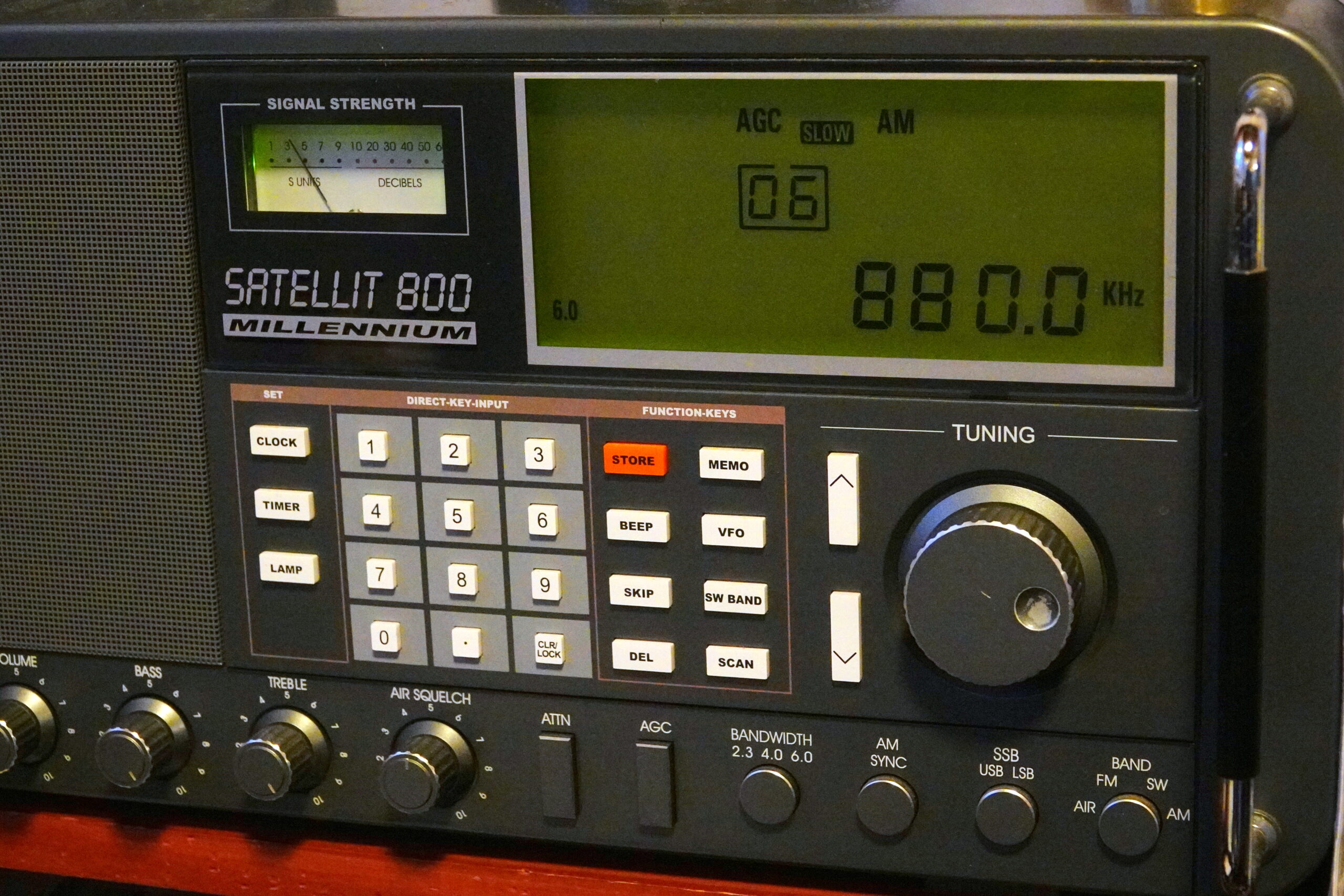
So what is it that Mr. Reitz did that set me off? Short answer: he wrote a really good article entitled “AM DX Antennas: Long Wires and Loops Big and Small.” In it, he mentioned that he could hear, from his location in Virginia, WCBS on 880 in New York City, some 300 miles away. He also mentioned that he could hear, during daylight hours, WGY in Schenectady, NY, about 400 miles distant.
WGY is a local station for me in Troy, NY, but I wondered: Could I hear WCBS in New York City? That’s nearly 150 miles from me. Hmmm.
So I started firing up various radios and radio/antenna combinations on 880 kHz. I tried my Icom IC706 MkIIIG ham transceiver, hooked to the 45-foot indoor end-fed antenna. Nothing heard.
Next, my Grundig Satellit 800 connected to its 4-foot whip antenna. I could hear WCBS barely, but with a horrible buzzing noise. Switching the Satellit 800 to the horizontal room loop antenna I could hear WCBS better, but the noise was really, really nasty.
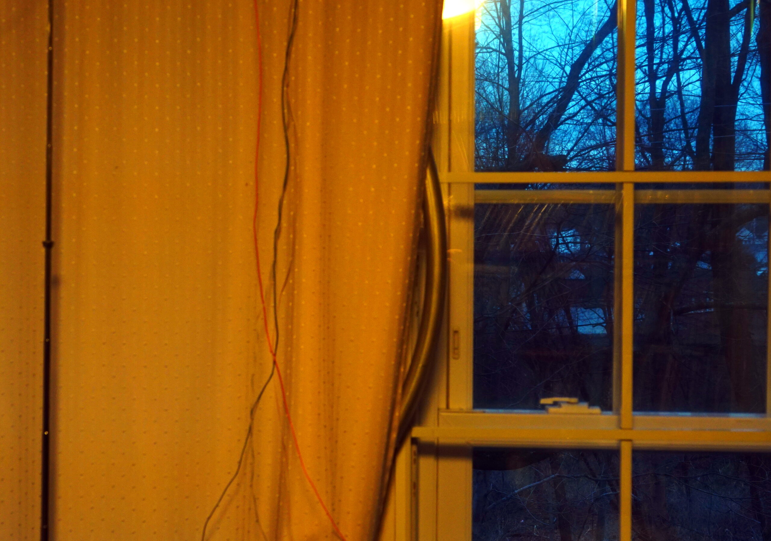
One way to preserve domestic tranquility is to hide the MFJ Loop behind a curtain!
Then I connected the MFJ 1886 Receive Loop Antenna. Tah-dah! I could hear WCBS just fine, with some noise in the background, but “armchair copy.” The MFJ loop made a huge difference in the quality and strength of the signal. I also tried the MFJ loop with another radio I have under test (its identity to be revealed in the future) and found, while I couldn’t hear WCBS at all with the radio’s internal antenna, the 1886 made an enormous difference, pulling out a fully copyable signal with noise in the background.
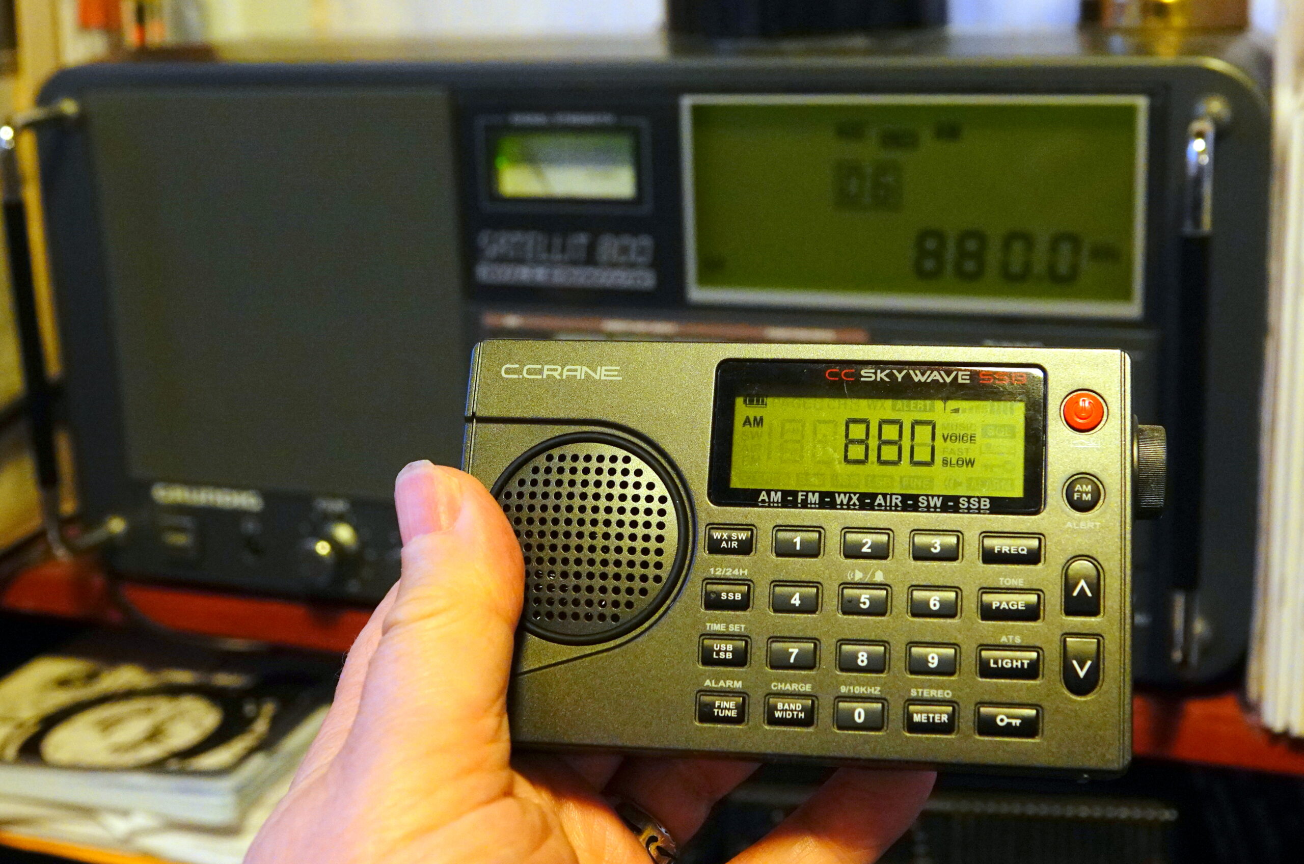 Finally, I tried a couple of my portables. My Tecsun 880 could hear WCBS, but the noise level was high enough to be annoying. Finally, I tried my CCrane Skywave SSB. The Skywave did a better job of pulling the signal out of the noise. I got the same result with the CCrane Skywave SSB2. Both Skywaves were using their internal ferrite antennas. Impressive.
Bottom line, for this very small foray into daytime medium wave DXing, the MFJ-1886 Receive Loop Antenna was a powerful and useful tool, one I can easily recommend. Second, when it comes to portables, the CCrane Skywave SSB (either model) continues to show that it is “The Little Radio That Could.”
Welcome to the SWLing Post’s Radio Waves, a collection of links to interesting stories making waves in the world of radio. Enjoy!
Bauer is removing Absolute Radio from Medium wave this month as it turns off all AM frequencies for the station across the country.
Absolute Radio launched exclusively on AM (as Virgin Radio) 30 years ago in 1993 using predominantly 1215 kHz along with fill-in relays on 1197, 1233, 1242 and 1260. Some of these have been turned off in recent years in places such as Devon, Merseyside and Tayside.
Whilst this is a historic milestone for the radio industry, it shouldn’t affect many listeners as just two percent of all radio listening currently takes place on AM.
Absolute Radio also lost its FM frequency in London in 2021 in favour of the ever-expanding Greatest Hits Radio network.
The move makes Absolute Radio a digital-only service, broadcasting nationally on DAB and online. [Continue reading…]
[…]Carlos Henrique Latuff de Sousa or simply “Carlos Latuff”, for friends, (born in Rio de Janeiro, November 30, 1968) is a famous Brazilian cartoonist and political activist. Latuff began his career as an illustrator in 1989 at a small advertising agency in downtown Rio de Janeiro. He became a cartoonist after publishing his first cartoon in a newsletter of the Stevadores Union in 1990, and continues to work for the trade union press to this day.
With the advent of the Internet, Latuff began his artistic activism, producing copyleft designs for the Zapatista movement. After a trip to the occupied territories of the West Bank in 1999, he became a sympathizer of the Palestinian cause in the context of the Israeli-Palestinian conflict and devoted much of his work to it. He became an anti-Zionist during this trip and today helps spread anti-Zionist ideals.
His page of Instagram (https://www.instagram.com/carloslatuff/) currently has more than 50 thousand followers, where of course you can see his work as a cartoonist and also shows his passion for radio. [Continue reading…]
A large and potentially dangerous sunspot is turning toward Earth. This morning (Jan. 6th at 0057 UT) it unleashed an X-class solar flare and caused a shortwave radio blackout over the South Pacific Ocean. Given the size and apparent complexity of the active region, there’s a good chance the explosions will continue in the days ahead. Full story @ Spaceweather.com ( https://spaceweather.com)
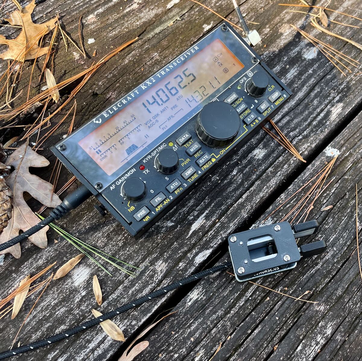
For almost 20 years, Steve Galchutt, a retired graphic designer, has trekked up Colorado mountains accompanied by his pack of goats to contact strangers around the world using a language that is almost two centuries old, and that many people have given up for dead. On his climbs, Galchutt and his herd have scared away a bear grazing on raspberries, escaped from fast-moving forest fires, camped in subfreezing temperatures and teetered across a rickety cable bridge over a swift-moving river where one of his goats, Peanut, fell into the drink and then swam ashore and shook himself dry like a dog. “I know it sounds crazy, risking my life and my goats’ lives, but it gets in your blood,” he tells me by phone from his home in the town of Monument, Colorado. Sending Morse code from a mountaintop—altitude offers ham radios greater range—“is like being a clandestine spy and having your own secret language.”
Worldwide, Galchutt is one of fewer than three million amateur radio operators, called “hams,” who have government-issued licenses allowing them to transmit radio signals on specifically allocated frequencies. While most hams have moved on to more advanced communications modes, like digital messages, a hard-core group is sticking with Morse code, a telecommunications language that dates back to the early 1800s—and that offers a distinct pleasure and even relief to modern devotees.
Strangely enough, while the number of ham operators is declining globally, it’s growing in the United States, as is Morse code, by all accounts. ARRL (formerly the American Radio Relay League), based in Newington, Connecticut, the largest membership association of amateur radio enthusiasts in the world, reports that a recent worldwide ham radio contest—wherein hams garner points based on how many conversations they complete over the airwaves within a tight time frame—showed Morse code participants up 10 percent in 2021 over the year before.
This jump is remarkable, given that in the early 1990s, the Federal Communications Commission, which licenses all U.S. hams, dropped its requirement that beginner operators be proficient in Morse code; it’s also no longer regularly employed by military and maritime users, who had relied on Morse code as their main communications method since the very beginning of radio. Equipment sellers have noticed this trend, too. “The majority of our sales are [equipment for] Morse code,” says Scott Robbins, owner of ham radio equipment maker Vibroplex, founded in 1905, which touts itself as the oldest continuously operating business in amateur radio. “In 2021, we had the best year we’ve ever had … and I can’t see how the interest in Morse code tails off.”
Practitioners say they’re attracted by the simplicity of Morse code—it’s just dots and dashes, and it recalls a low-tech era when conversations moved more slowly. For hams like Thomas Witherspoon of North Carolina, using Morse code transmissions—sometimes abbreviated as CW, for “continuous wave”—offers a rare opportunity to accomplish tasks without high-tech help, like learning a foreign language instead of using a smartphone translator. “A lot of people now look only to tools. They want to purchase their way out of a situation.”
Morse code, on the other hand, requires you to use “the filter between your ears,” Witherspoon says. “I think a lot of people these days value that.” Indeed, some hams say that sending and receiving Morse code builds up neural connections that may not have existed before, much in the way that math or music exercises do. A 2017 study led by researchers from Ruhr University in Bochum, Germany, and from University Medical Center Utrecht in the Netherlands supports the notion that studying Morse code and languages alike boosts neuroplasticity in similar ways. [Continue reading…]
Please consider supporting us via Patreon or our Coffee Fund!
Your support makes articles like this one possible. Thank you!

 Many thanks to SWLing Post contributor Loyd Van Horn at DX Central who shares the following announcement:
What a great season of DX Central Live! and the MW Frequency Challenge it has already been and we are just getting started! This season, you helped us cross 1,000 subscribers on our YouTube channel, have brought in a record number of MW Frequency Challenge submissions thus far, and have helped to generate a lot of energy around this DX season! We couldn’t do it without your support, so thank you!
First, a little housekeeping. We will be taking some time off to spend the holidays with family and of course – some DX! As such, there will be no DX Central Live! on Friday, December 23 or 30th. We will return on Friday, January 6, 2023.
Also during this time, we will be taking a brief pause on our weekly MW Frequency Challenge as well. I will be announcing the results from week 12 (576-600) when we return on Jan 6, as well as the next frequency range at that time.
Don’t worry, we have a challenge for our little break that should provide all of the fun and difficulty to push DXers to scratch new ones in their logbooks: The Inaugural DX Central MW Daytime Challenge.
The premise: Log as many stations as you can during daytime conditions. That’s it!
Nothing but daytime DX (period from 2 hours after local sunrise to 2 hours prior to local sunset) starting at 0200 UTC Saturday, December 17 and ending at 0200 UTC Monday, January 2, 2023. This challenge is open to all DXers around the world!
A few rules:
– Loggings must be during your local daytime period (2 hours after local sunrise to 2 hours prior to local sunset)
– Loggings must be from between 0200 UTC Saturday, December 17th and 0200 UTC Monday, January 6.
– Any stations are allowed for this challenge: local stations, TIS/HAR, part 15 transmitters not to mention anything distant you might be able to pull in!
– Stations do not need to be “new to you”, relogs are allowed
– Stations need to be on any mediumwave frequency between 530-1710 kHz.
– Loggings should be from a location within 50 miles of your home location. This includes use of online SDRs, portable operations, etc.
– If you are traveling for the holidays and will be away from home but have access to either your station remotely or another online SDR from your home location, those submissions will be allowed.
– Only submissions made using the Google Form sheet (link below) will be considered for the challenge. Social media posts, emails, etc will not count.
Categories for this challenge will include US and international versions of:
– Most stations logged
– Most US States/Canadian Prov logged
– Most countries logged
– Furthest reception
– Most frequencies with at least one logged station
Google Form for entries: https://forms.gle/TVgCPrHMpfDAzbzb6
I hope this challenge will be a fun one for all!
To all of our fellow DXers, supporters, family, friends….Merry Christmas, Happy Holidays and may your logbooks be filled with DX and your hearts filled with joy and love!
73,
Loyd Van Horn
W4LVH – Mandeville, LA
 Many thanks to SWLing Post contributor, Giuseppe Morlè (IZ0GZW), who writes:
Dear Thomas and all friends of the SWLing Post,
I’m Giuseppe Morlè from Formia on the Tyrrhenian Sea…
I wanted to share this experiment of mine with all of you by tuning the medium waves with two separate loop cassettes and each for itself by exploiting the principle of induction between two conductors placed next to each other.
I superimposed one cassette on the other by matching the windings of the medium waves–each variable works only for its own box.
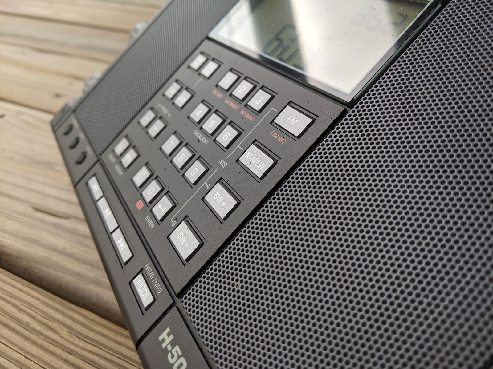
I’m tuning the Algerian JIL FM station on 531 kHz with the Tecsun H-501X connected to the box below…then, passing to the top box, the one without any physical contact with the receiver, I tuned this station again centering it perfectly thanks to the induction that creates between the two close windings.
My video will clarify any doubts and I would like to receive your comments about it.
My constructions are the result of continuous recycling and spending very little to get a good yield.
You can view this video below or on my Youtube channel:
[Note that you can translate this video into your language via YouTube’s automatic subtitles. Click here to learn how to do this.]
I’m available for any clarification…
Thanks to all of you and I wish you good listening.
73. Giuseppe Morlè iz0gzw.
Thanks so much for sharing your antenna experiments with us, Giuseppe!