Many thanks to SWLing Post contributor Nick Hall-Patch, who has kindly provided a translation of this article from the Japanese-language publication PROPAGATION by the Totsuka DXers Circle (TDXC). In this piece, Satoshi Miyauchi explores how WavViewDX can revolutionize SDR analysis by making propagation and reception conditions instantly visible–and shares some remarkable reception examples.
“Ultra” Convenient, The Benefits of WavViewDX: Visualizing Reception Conditions
by Satoshi Miyauchi
After recording bands using SDR’s such as Perseus or HF Discovery, I was informed by Kazu Gosui via email of a new program that’s “ultra” convenient for analyzing them. When monitoring in real time with Perseus, I have a general memory and notes of what was received at what time. However, when recording reception data without real-time monitoring, such as during nighttime hours, verifying and analyzing the data across all frequencies takes time. Knowledge and intuition about where to listen are also important elements. While all of this is a skill, I believe that previous tools have been unable to provide a comprehensive view of the day’s conditions. Since I started using WavViewDX, I’ve been using it every morning, efficiently analyzing the SDR recordings I’ve collected.
By the way, recently I’ve been using a timer (the “Scheduler” of SDR Console) to check if the TWR-Africa signal transmitted from Benin, West Africa, is reaching me in the middle of the night. My analysis showed a significant reduction in the time required for confirmation that TWR-Africa was being received before and after WavViewDX was installed, and I’d like to share this with you.
Just to be clear, this article is not intended to be a tedious rehash of the user manual. Rather, it is intended to provide useful, pinpointed tips for use.
- I’ll introduce a method I think might be best based on my current setup.
- I’ll share some reception reports from my recent morning routine.
- I’ll touch on the mysteries of radio wave propagation, a realization I believe is unique to WavViewDX.
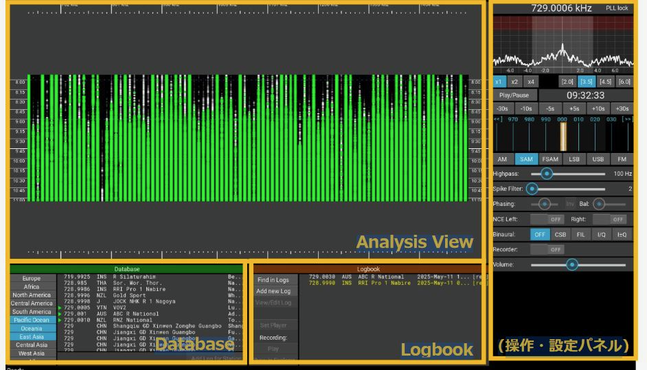
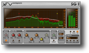
But first, a word about WavViewDX: seeing is believing. As shown in the sample image in Figure 5, it visually displays the status of stations received at each frequency, using green bars or white lines, in chronological order, from the lowest frequency band (left) to the highest (right). You can even customize it to analyze North and South America at 10 kHz intervals for TP reception.
The author is Reinhard Weiß from Germany (please see accompanying related articles). It is an incredibly easy-to-use and intuitive software. Once you start using it, you’ll definitely want to keep it.
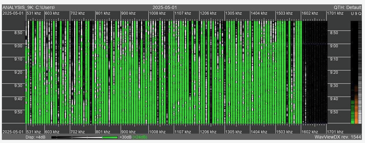
Figure 5
First, let’s assume you’ll be importing and analyzing data into WavViewDX.
1.) Timer Reception Tips, Using SDR Console
This is a backward-thinking approach based on the fact that WavViewDX can import files in “folders.” The golden rule is simply to store all files from a single session in a single folder. I’ve been using SDR Console as my primary SDR program for a while now, so when I register a scheduler (for timer scheduling), I click “Add date (yyyy-mm-dd) subfolder” under “Folder”, in Figure 6. This allows me to import the entire folder of recording files from that day into WavViewDX, saving me a lot of time. WavViewDX has a “Select Whole Folder” button, which allows me to import files into WavViewDX with a single click (Figure 7). How amazing! Incidentally, I set up bandwidth recording files to be stored in separate 1GB files. The moment I wake up, the files are instantly imported into WavViewDX, allowing me to quickly check the conditions from midnight to dawn before work.
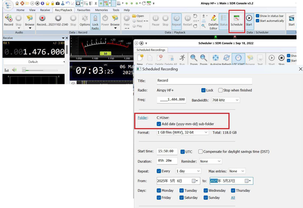
Figure 6
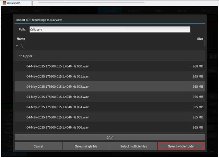
Figure 7
2) TWR-Africa Reception Recording
Even on shortwave, it’s rare to see signals from Africa, let alone on mediumwave. Until a few years ago, I thought this was impossible. However, I discovered that I could record pre-dawn signals from Africa on my home K9AY loop, including the VOA of the Sao Tome and Principe relay on 1530kHz, as well as the famous TWR Africa (Benin) on 1476kHz. Of course, it’s not easy to receive signals every day, so I was not motivated to record them regularly However, after installing WavViewDX, I was able to easily grasp the pre-dawn conditions, and I set up a scheduler to record as many times as possible every day.
Then, one morning, right around 3:30 AM, on the morning of the March vernal equinox, I noticed a very clear bar on the 1476kHz using WavViewDX (Figure 8). By working in conjunction with WavViewDX, it automatically checks offsets in exact carrier frequency being received against the MWList database, and the > mark quickly lights up in WavViewDX, indicating that it’s TWR Africa! I was surprised when I heard the audio. I was impressed by the exceptionally clear reception. There was a slight beat, and it seemed like at least one other carrier was also in the mix. How such clear audio managed to reach and be heard across nearly 13,300 km as the crow flies is a mystery, but it’s still a moving experience.
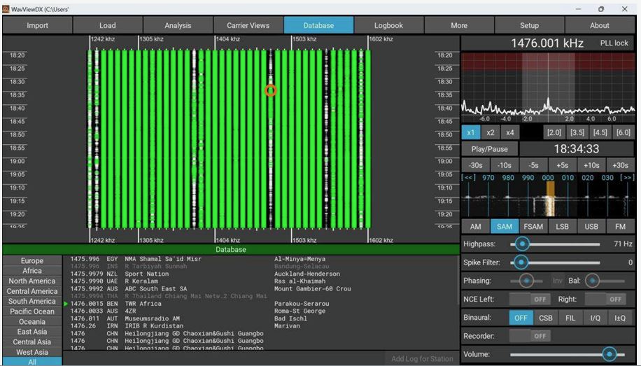
Figure 8
I asked @lft_kashima LFT Kashima Fishing Radio, who regularly posts information on X, and he said that the signal wasn’t as good on that day at his location. Since we’re both in the Kanto region and a little farther apart, perhaps that’s the problem, or perhaps it’s just the antenna. He uses a north-south loop antenna, while I use a vertical AOR SA-7000.
While I don’t know the full reason or answer, one possible guess: – Wasn’t the arrival direction north-south? – Did it arrive through a duct somewhere? However, there’s no way to know why the duct ended up at this receiving point. It’s a wonder that I was able to receive such a DX station at this point in the solar cycle, when the number of sunspots is almost at its maximum and the A/K Index was far from calm. This makes daily reception all the more meaningful. It’s a moment that makes me admire nature, the work of radio wave propagation. I was able to receive this station again in April, and the links to those two results from 1476kHz – TWR Africa are below:
- Received Audio 1: March 19, 2025, 18:35 UTC https://youtu.be/gWORriKCJ7c
- Received Audio 2: April 14, 2025, 18:31 UTC https://youtu.be/DfYn-gbp2SY
3) The Mysteries of Radio Wave Propagation Discovered Only with WavViewDX
WaveViewDX already clearly shows the reception status on the vertical time axis, but just before the vernal equinox, a phenomenon in which the propagation conditions deteriorated simultaneously across multiple frequencies occurred, albeit for a short period of time. (Audio Sample https://youtu.be/XhXSQFiGQeo) What is this? Figure 9 shows the actual situation at my location on March 17, 2025, after 18:00 UTC.
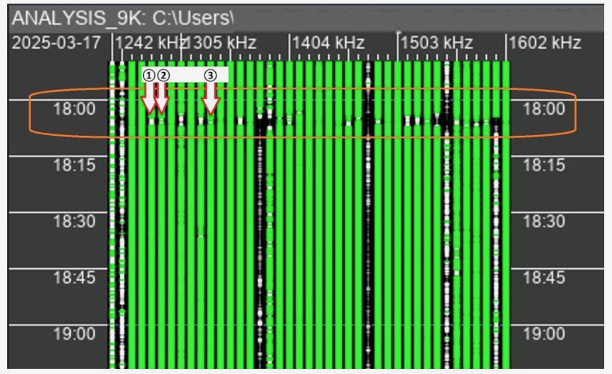
Figure 9
- 1278kHz JOFR Fukuoka RKB Mainichi Broadcasting System 50kw (about 900km distance, 245°)
- 1287kHz JOHR Sapporo HBC Hokkaido Broadcasting System 50kw (about 1000km distance, 340°)
- 1332kHz JOSF Nagoya Tokai Broadcasting System 50kw (about 270km distance, 270°)
(*Note: The leftmost bar (1242kHz in the Kanto region) is attenuated with a notch filter)
One of the benefits of WavViewDX is that it visually showed the simultaneous drop in signal strength from domestic and international stations, which had been arriving almost smoothly until 18:00 UTC.
I asked Perplexity AI and searched the literature. These possibilities were listed:
“Regarding the phenomenon of simultaneous attenuation of radio signals in all directions for several minutes during nighttime propagation in the medium frequency band (MF band),” it is believed to be primarily caused by the combined effects of the following factors: –
- Ionospheric Variation Mechanism Sudden E-Layer (Es-Layer) Formation A localized increase in electron density in the upper E-layer of the ionosphere (at an altitude of 100-120 km) at night. This thin ionosphere strongly reflects signals, blocking the normal F-layer reflection path. One measurement data showed signal attenuation of up to 20 dB when the Es layer occurred.
- F-layer altitude fluctuations: When the F layer (altitude 250-400 km), the main nighttime propagation path, rapidly rises due to thermal expansion, the reflection angle changes, creating a “propagation hole” that causes signals to deviate from the receiving point.
- Earth’s magnetic field fluctuations disrupt the electron distribution in the ionosphere, causing a sudden increase in absorption.
- Instantaneous changes in solar activity: The emission of X-rays and charged particles associated with solar flares suddenly changes the electron density in the ionosphere, destabilizing the reflection coefficient and resulting in short-term propagation loss.
Although it was able to provide various possible explanations, I was unable to perform any further verification of these answers myself.
These English translations were prepared for IRCA’s DX Monitor, and are used with the kind permission of IRCA as well as of the authors and the editor of the Totsuka DXers Circle publication, PROPAGATION.