My NCPL antenna

Many thanks to SWLing Post contributor, Grayhat, who shares the following modification he made to a Noise-Cancelling Passive Loop antenna last year. He’s kindly allowed me to share his notes here, but apologized that at the time, he didn’t take photos of the project along the way and recycled many of the components into yet another antenna experiment.

Grayhat writes:

Here’s a simple tweak to the NCPL, made easy for anyone. Let’s start with the commercial NooElec 9:1 balun version 1 (not 2) … made in USA.

Look at the schematic of the balun:

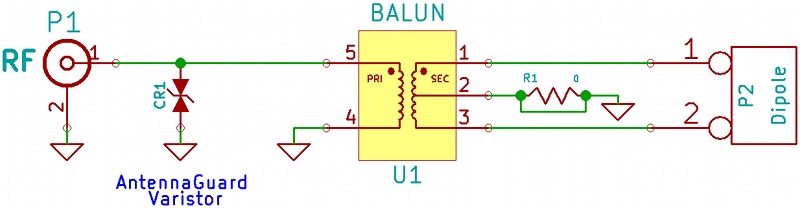
Cut the R1 (0 Ohm resistor – jumper) so that the center tap of the transformer won’t be connected to ground, then solder a short piece of wire to the tap.

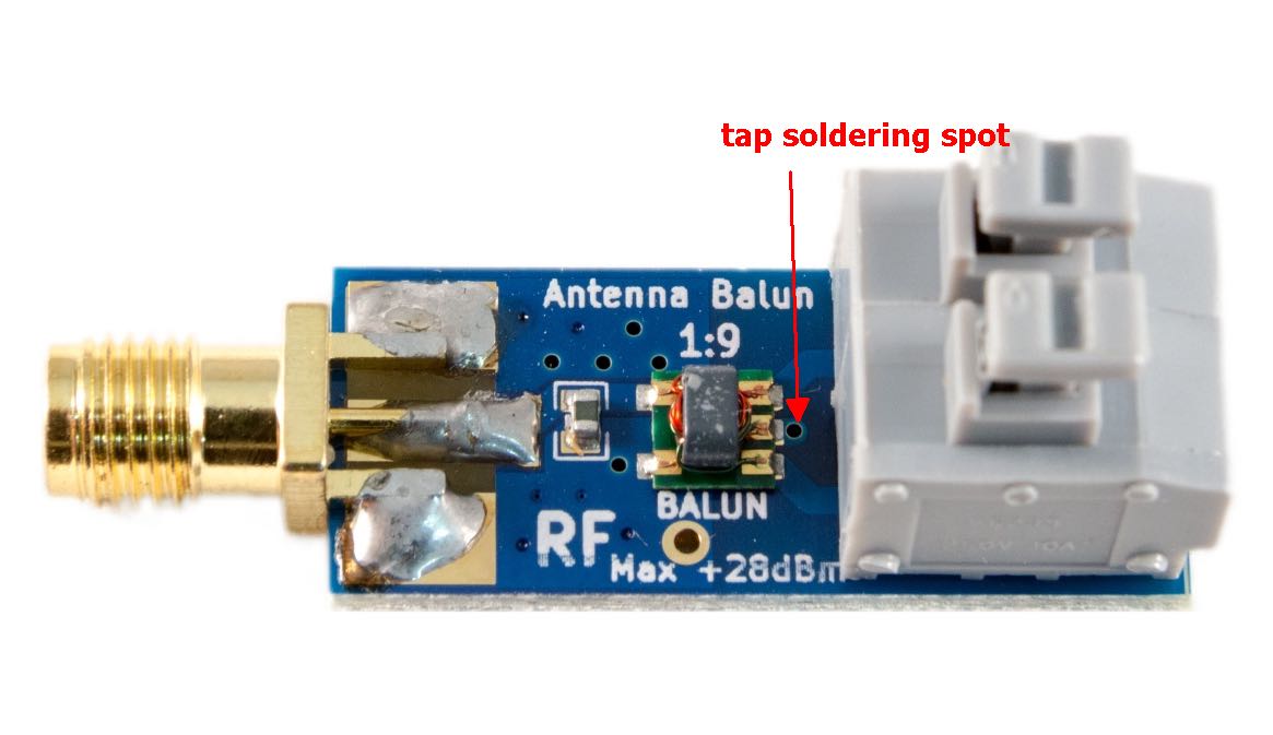
The first pic (top) shows the balun seen from top side, the arrow indicates the small hole going to the transformer tap.

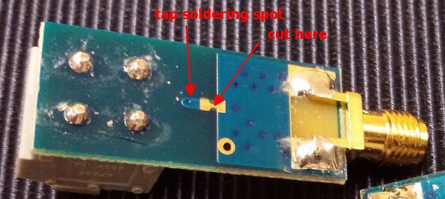
This pic shows the bottom of the board with the trace to cut and the spot for soldering the tap wire (needs cleaning with a bit of sandpaper to remove the cover paint). The solder is as easy as 1-2-3 once the trace is cut and the spot cleaned just insert a wire from the top of the board and solder it to the bottom and there you go!

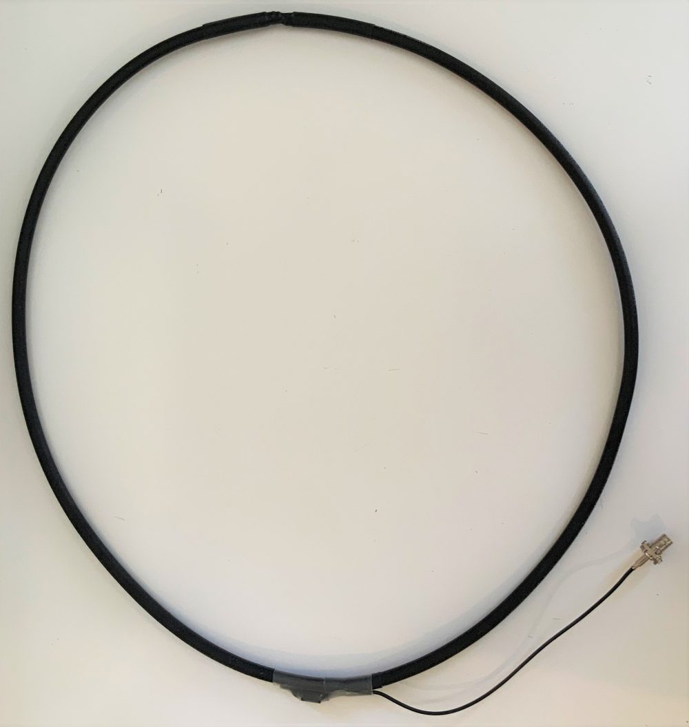
Build the NCPL using “fat” coax (RG8 will do) with the top cross connection.

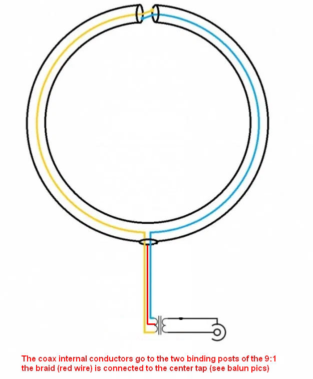
NCPL modification schematic

Side note: the top “cross connection” is the weak point, so it would be a good idea putting a short piece of (say) PVC pipe over that point, the piece will also help suspending the loop or sticking its top to the support pole, as for the feedpoint, a small electrical junction box will fit and protect the tiny balun from bad weather

Now the difference: connect the two center conductors of the NCPL to the balun input and the braid to the wire going to the center tap (as above).

Such a configuration will give some advantages over the “standard” NCPL one. The loop will now be galvanically isolated from the feedline/receiver so it will have much less “static noise.” Due to the tap, the typical 8 pattern of the loop will be preserved, this means that the loop will now have much deeper nulls.

By the way, the balun could just be wound w/o buying it. I suggested the nooelec since that way anyone with little soldering ability will be able to put it together. Oh and by the way it’s then possible adding a small preamp at the balun output if one really wants, any preamp accepting a coax input will work. 🙂

Again, if you can/want, give it a try !

Many thanks for sharing this, Grayhat! We always welcome your inexpensive, innovative urban antenna projects!

Post readers: If you have question, feel free to comment and I’m sure Grayhat can help.