Many thanks to SWLing Post contributor, Bill (WD9EQD), who shares the following guest post:

Time Shifting Radio Programs for Later Listening
by Bill (WD9EQD)
There are quite a few programs on shortwave that I enjoy listening to for the actual program content. If I am lucky, I will receive a strong enough signal to really enjoy the experience. But all too often, I either can’t directly receive the program or conditions are such that listening is just not enjoyable. What I was looking for was good quality sound that I could listen to on my schedule.
I could always just go to the station website and listen to the live stream of the program. But what if there are two programs on different stations at the same time? I would have to choose which one to listen to. What I needed was a way to listen to the program on my schedule.
This write-up will be presenting several ways this can be accomplished.
Is the Program Streamed?
In many cases, it is possible to go to the program’s website and then listen to the latest program or even an archive of past programs at your convenience. Some examples are:
 Hobart Radio International http://www.hriradio.org/
Radio Emma Toc https://www.emmatoc.org/worldserviceindex
VORW International https://soundcloud.com/vorw
AWR Wavescan http://eu.awr.org/en/listen/program/143
Blues Radio International: http://www.bluesradiointernational.net/
This is a Music Show https://thisisamusicshow.com/
Radio Northern Europe International: https://www.mixcloud.com/RadioNorthernEurope/
Alt Universe Top 40: https://www.altuniversetop40.com/links
International Radio Report https://www.ckut.ca/en/content/international-radio-report
World of Radio http://worldofradio.com/
The Shortwave Report http://www.outfarpress.com/shortwave.shtml
Lost Discs Radio Show https://www.lostdiscsradio.com/
Grits Radio Show https://archive.org/details/gritsradioshow2020
Le Show with Harry Shearer http://harryshearer.com/le-show/
Can the Program Be Downloaded?
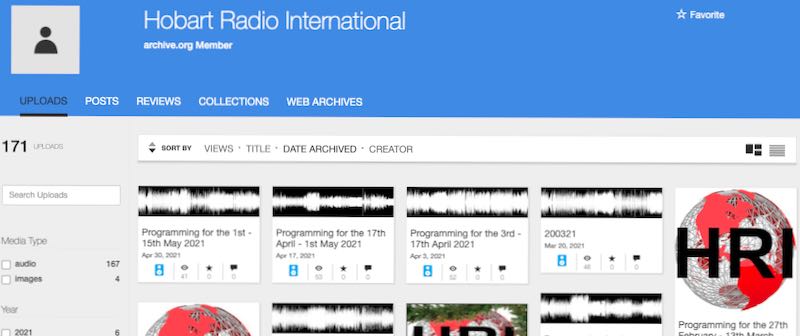
All HRI programs are available on their Archive.org page.
Quite often, the program’s web site will also let you download the program for listening at a later date. Some examples are:
Hobart Radio International has an Internet Archive page where you can listen to and download their previous programs: https://archive.org/details/@hobart_radio_international
Radio Emma Toc has a button for “broadcast & internet relay services wishing to air our programme”.
But anyone can download the program.
VORW International: https://soundcloud.com/vorw
(Note: You will have to sign into Soundcloud to be able to download the files)
AWR Wavescan: http://eu.awr.org/en/listen/program/143
Your Weekend Show: https://open.spotify.com/show/2RywtSHWHEvYGjqsK6EYuG
International Radio Report https://www.ckut.ca/en/content/international-radio-report
World of Radio http://worldofradio.com/
The Shortwave Report http://www.outfarpress.com/shortwave.shtml
Lost Discs Radio Show https://www.lostdiscsradio.com/
Grits Radio Show https://archive.org/details/gritsradioshow2020
Le Show with Harry Shearer http://harryshearer.com/le-show/
WBCQ has a link to an Archive of some of their programs. Just click on the Archive link and you will go to Internet Archive where there are a lot of programs that can be streamed or downloaded. The programs include:
- Adventures in Pop Music
- Analog Telephone Systems Show
- B Movie Bob
- Cows in Space
- Godless Irena 1
- Grits Radio Show
- Lost Discs Radio Show
- Radio Timtron Worldwide
- Texas Radio Shortwave
- The Lumpy Gravy Show
- Zombies in your Brain
- Vinyl Treasures
- Plus many, many other programs…
Does the Program Have a Podcast?
Check to see if the program has a podcast. Many programs do and this makes it easy to always have the latest program updated into my favorite podcast program.
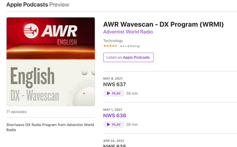
AWR Wavescan is available on a number of podcasting platforms
Some programs that have podcasts:
- Hobart Radio International
- AWR Wavescan
- Blues Radio International:
- Your Weekend Show
- International Radio Report
- World of Radio
- The Shortwave Report
- The Lost Discs Radio Show
- Le Show with Harry Shearer
Directly Record the Stream While It Is Being Broadcast
This method is a little more difficult and requires some setup. The method is to record the program directly from the internet stream of the station as it is broadcasting the program. Once set up, the procedure is completely automatic and will continue to capture the program until it is disabled in the scheduler.
Let’s walk through a typical program that we want to record. I like Alan Gray’s “Last Radio Playing” program on WWCR. It is broadcast weekly on Wednesday at 6pm Central Time on 6115. While I can receive the program over the air, it’s not very good reception, so I usually just stream it off the internet.
What I want to do is to set up an automatic computer program that will connect to the stream on Wednesday night, record the stream for one hour and then disconnect. I use the program StreamRipper which can run on either Linux or Windows.
http://streamripper.sourceforge.net/
Since I have a spare Raspberry Pi 4 computer, I chose to use the Linux version. The following description is based on Linux. A similar method I’m sure could be done with the Windows version.
Fortunately, StreamRipper is in the current software repository for the Raspberry PI and I could just install it with having to do a compile. I’m sure other Linux distributions probably also have it in their repository. It was a simple matter to install it. In Linux, Streamripper is run from the command line in a terminal window.
A typical command line for SteamRipper is:
streamripper station_URL_stream –a “filename” –A –d directory_path -l seconds
where
station_URL_stream is the http address of the audio stream. Determining this can sometimes be challenging and some methods were recently discussed in a SWLing Post:
https://swling.com/blog/2021/04/robs-tips-for-uncovering-radio-station-stream-urls/
–a says to record the audio as a single file and not try to break it up into individual songs.
“filename” the filename of the resultant mp3 file goes here in quotes
-A again says to create a single file.
-d tells it the directory path to store the mp3 file. Place the full directory path after the –d
-l specifies how long to record. Enter the number of seconds after –l.
(note: this is lower case letter l)
For Last Radio Playing, the command line is:
streamripper http://67.225.254.16:3763 –a “Last Radio Playing” –A –d /home/pi/RIP/wwcr –l 3600
when executed, this would connect to the URL stream, record for 3600 seconds (60 minutes) and then disconnect from the stream A file called “Last Radio Playing.mp3” would be in the wwcr1 directory.
Save this command line to a shell file, maybe wwcr.sh. Then make this shell file executable.
Last is to enter a crontab entry to schedule the shell file wwcw.sh to be run every Wednesday at 6pm ct.
At the command line, enter crontab –e to edit the cron table.
Add the following line at the end:
0 19 * * 3 /home/pi/wwcr.sh
then exit and save the crontab file.
This line says to execute wwcr.sh every Wednesday at 1900 (my computer is on eastern time).
There are many ways to enhance the shell script. For example, I have added the date to the mp3 file name. My wwcr1.sh shell script is:
NOW=$(date +”%Y-%m%d”)
# WWCR1 Last Radio Playing
# Wednesday 7-8pm et
streamripper http://67.225.254.16:3763 -a “$NOW Last Radio Playing” -A -u FreeAmp/2.X -d /media/pi/RIP/wwcr1 -l 3600
This will create a MP3 file with the date in the file name. For example
2021-0505 Last Radio Playing.mp3
Note: I named the file wwcr1.sh to denote that WWCR transmitter 1 was being streamed. Each of the WWCR transmitters have different stream URL.
Most radio streams work fine with the default user agent but WWCR required a different user agent which is why the –u FreeAmp/2.X is added. Normally, –u useragent is not required. The default works fine.
For each program, just create a similar shell file and add it to the cron scheduler.
Streamripper is very powerful and has many options. One option is for it to attempt to divide the stream up into individual files – one for each song. Sometimes this works quite well – it all depends on the metadata that the station is sending over the stream. I usually just go for a single file for the entire show. Some stations are a little sloppy on whether the program starts on time – sometimes they start a minute early and sometimes run a minute over. The solution is to increase the recording time to two minutes longer and then specify in the crontab file that the show starts a minute early. It’s easy to adjust to whatever condition might be occurring.
Recording the BBC
I have found that the BBC makes it more difficult to use this procedure. For one thing, they have just changed all their stream URL’s. And they have decided NOT to make them public. When they did this some of the internet radios broke since they still had the old URL’s. Of course it didn’t take long for someone to discover and post the new stream URL’s:
https://gist.github.com/bpsib/67089b959e4fa898af69fea59ad74bc3#file-bbc-radio-m3u
I have tested the Radio 4 Extra stream and it does seem to work. For how long is anyone’s guess.
I found that while streamripper did seem to work on BBC, all the mp3 files came out garbled. So the method above doesn’t seem to work with the BBC.
I went back to the drawing board (many hours on Google) and discovered another way to create a shell script that can be scheduled to record a stream. This involves using the programs mplayer and timelimit.
First step is to install the programs mplayer and timelimit to the Linux system. mplayer is a simple command line audio and video player. timelimit is a program that will execute another program for a specific length of time.
First I created a shell script bbc30.sh:
#!/bin/bash
NOW=$(date +”%Y-%m%d-%H%M”)
# BBC Extra 4 – 30 minute program
timelimit -t1800 mplayer http://stream.live.vc.bbcmedia.co.uk/bbc_radio_four_extra -dumpstream -dumpfile /media/pi/RIP/$NOW-bbc.mp3
Note: The bold line above is all on one line in the shell file.
This script will execute the timelimit command. The timelimit command will then execute the mplayer command for 1800 seconds (30 minutes).
The mplayer command then connects to the http stream; the stream instead of playing out loud is dumped to the dumpfile /media/pi/RIP/$NOW-bbc.mp3
The crontab entry becomes:
30 23 11 5 * /home/pi/bbc30.sh
In this case, the program on May 11 at 2330 will be recorded.
Summary
In conclusion, Podcasts are the easiest way to get the programs. But automatically recording directly from the station stream is really not that much harder to do. Just be careful. It’s very easy to accumulate much more audio than you can ever listen to in this lifetime.
One final note. The use of a Raspberry Pi makes this a very easy and convenient method. I run the pi totally headless. No keyboard, mouse or monitor. It just sits on a shelf out of the way and does it thing. I either log in using VNC when I want the graphical desktop, Putty for the command line, or WinSCP for transferring files. The Pi stays out of the way and I don’t end up with another computer system cluttering up my desktop.
Besides recording several shortwave programs, I use Streamripper to record many FM programs from all around the United States. It’s great for recording that program that is on in the early morning hours.
73
Bill WD9EQD
Smithville, NJ
Thank you for sharing this with the SWLing Post community, Bill! This weekend, I’m going to put one of my RPi 3 units into headless service recording a few of my favorite programs that aren’t available after the live broadcast. Many thanks for the detailed command line tutorial!


")