Many thanks to SWLing Post contributor and WWLG author, John Figliozzi, who shares the following review:
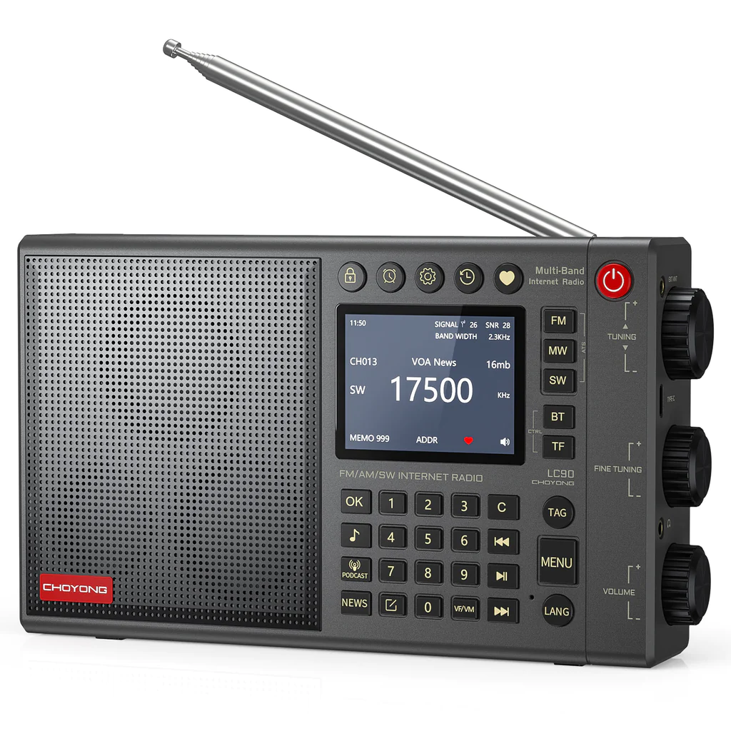
A Review And Analysis Of The Choyong LC90 (Export Version)
By John A. Figliozzi
General
To my knowledge, this is the first radio to combine AM Shortwave with Internet Radio. This makes it the first true “full service” radio incorporating ALL of radio’s major platforms. Many radio listeners question why this hasn’t been done sooner, so this very good first effort is most welcome.
The initial presentation of the radio to the new owner is impressive. The stylish box in which it arrives is worthy of a respected instrument of high quality. The radio has the solid substantial feel of a device with excellent build quality. Its sizing – that of a paperback book along the lines of some previous well-respected AM/FM/SW receivers like the Grundig YB-400 – gives it the perfect form factor for a radio that can be enjoyed both in the home and as a portable.
There is so much to like here. Over and above its unique combining of Internet radio and shortwave, there’s a “permanent” battery that offers many hours of use before it needs recharging, ATS tuning, the ability to save frequencies and stations in several preference lists, several ways of searching for Internet radio stations, an easy way to add Internet stations not already listed by the manufacturer, and others.
But the LC90 really shines with its fantastic audio on FM and Internet radio. There’s a woofer, a tweeter and a low frequency diaphragm inside the speaker cavity that occupies the left half the case – and nothing else. The radio’s excellent build quality and its developers’ efforts to produce a world class audio section in a portable radio really pays off.
But no radio is perfect, and this one obviously is a work in progress. So, being critical – which is what a review and analysis like this does — should not imply disapproval on any level. On the contrary, the LC90 is already a well-formed radio worthy of consideration by any purchaser.
The Screen
The screen that is the center of the LC90 provides much information depending on the platform being used. But in some cases, useful information is missing and in other cases the information provided seems unnecessary or of questionable utility.
In AM (MW), FM and SW, it is not readily apparent what all the symbols mean or why they are there. The time, signal strength and SNR (signal to noise ratio), bandwidth, meter band, heart (for including a frequency in “favorites”) and the “Freq. vs. Addr.” indicators are all helpful and understandable. But what is meant by “Memo” isn’t entirely clear. Is it holding just my preferences? Or the number of stations found by ATS? Or something else?
So, too, with the Internet Radio screen. What do the three dots, the speaker icon and the return icon mean? The ability to tune stations in sequence as they appear across the bottom of the screen depending on mode is both unique and helpful. But the use of a timer to tick off how long one might listen to a particular station seems of dubious value.
Some suggestions for better use of the screen in some circumstances are detailed below.
Operation
Initial setup matching the radio to home internet service proceeded flawlessly. The time clock is in 24-hour mode and showed correct time and date in my time zone. Some purchasers had previously noted that the clock showed a time one hour earlier than the actual time. I surmise that this is because the clock remains in standard time year-round. There is no facility to reset the clock, compensate for seasonal time changes or set the clock manually. This is an oversight that should be addressed.
This is a sophisticated, multi-faceted radio. As impressive as it already may be, it should be perceived as a work in progress in need of the improvements it will get eventually through firmware updates and design modifications. It would be helpful if those updates could come directly and seamlessly through the Internet, something that apparently can’t be done currently.
The LC90 comes with a rather short, almost cryptically worded pamphlet. This can serve as an ok quick start-up guide. But after using the radio, it’s obvious that there’s need for a comprehensive operation manual with copious directions for the user, along the lines that Eton provided for the E1. A radio of this quality and at this price point demands such consideration.
In short, becoming fully familiar with and comfortable using all the features of the LC90 requires a prodigious learning curve, one that is not intuitively discerned. I have to say that even after using it almost constantly for a few weeks, I feel I am still missing things.
Just a few examples of aspects that go unexplained include:
- What does “Auto Play” mean in Settings?
- Getting to preferences (the “heart” icon) is confusing and I’ve inadvertently removed them without learning how it happened.
- Why does the screen show “Please add radio channel first” when I think I’ve already done that?
- Why does screen alarmingly show “Saved channels removed”, having done so when I press the tuning dial thinking I am obtaining a list of my preferred or saved stations?
The cleverness behind the LC90 is not intuitively apparent. If I hit the wrong keys in combination or hard press instead of soft press a key, I get a result I don’t understand and for which there is no explanation in the exceedingly short manual provided now. In some cases, I put myself in a corner I can’t get out of, so I must reset by shutting down and restarting the radio to get back to base.
Following are my observations on the performance of the LC90 by platform:
FM
The LC90 has a very good FM section that is quite sensitive. Using the ATS feature, (automatic tuning) it found 37 stations in Sarasota FL, for example.
For its size – and even considering many larger radios — the LC90 has an excellent audio response on FM. However, although it has activated stereo capability, it does not appear to actually provide stereo through its ear/headphone jack. This is because the same output is used to provide audio to the speakers and the ear/headphone jack. This feels like an oversight that should be rectified. The radio does “recognize” a stereo plug and audio does play into both ears. It’s just not stereo audio.
As currently configured this LC90 does not offer RDBS (RDS in Europe) on FM. This should be incorporated into a radio of this quality being offered at this price point.
Even so, in this user’s opinion it earns a 4.5 on scale of 5 on FM. But if it had stereo and RBDS, it would easily earn a 5.
A question arises: Were HD Radio (in North America) and DAB+ (in Europe and Australia – if these are targeted markets for the LC90) considered for incorporation into this radio by its developers? If not, why not; and, if so, why was a decision taken not to include them?
Shortwave
Performance of the LC90 on shortwave is very good, especially since it clearly is not intended as a hobbyist’s DX machine. As such in my opinion, it doesn’t require the SSB capability that some have said they wish it has.
Rather, this radio is intended for the content-focused listener. I view the AM (MW), FM and SW platforms as back-up alternatives for and secondary to the primary focus — Internet Radio. Nonetheless, the LC-90’s performance is above average on both FM and SW which should be assuring to anyone considering its purchase.
The LC90 is quite sensitive on SW for a small portable using just its built-in expandable and rotatable 9 stage rod antenna. But it does especially well when a common clothesline reel external antenna is extended and plugged into the receptacle provided for that purpose on the radio’s right-hand side. (Similar improvement is noted for AM (MW) and FM, as well.)
Complaints about placement of this receptacle close to the tuning knob is of no concern when an external antenna of the type described above using a 3.5mm plug connector is used. Any more sophisticated an external antenna would likely overload this radio considering that “birdies” – false signals internally generated by the radio itself — can be detected throughout the SW spectrum even when just using its built-in rod antenna. This flaw should be addressed in any future modification or upgrade.
The audio enhancements made on this radio through unique use of speakers and their orientation are not as apparent here as they are when listening to FM and Internet Radio.
On AM signals generally — both SW and AM (MW) – a listener can detect artifacts in the audio. Audible random “clicks” often can be heard – usually when receiving weaker stations – which sounds as if the radio’s audio section is clipping. Adjusting the bandwidth appears to offer only minimal help with this.
Indeed, the audio produced by SW and AM (MW) sounds somewhat mechanical except on very strong stations. It seems to lack body or depth on SW and AM. Some of this undoubtedly is due to the quality of AM audio to begin with. But the latter does sound more natural on other receivers. The 7 bandwidths provided (1, 1.8, 2, 2.5, 3, 4, 6 kHz) do help to somewhat shape the audio, but it appears that there could be better choices for what this radio is trying to achieve.
Nonetheless on SW, the LC90 rates a comparative 3.75 on a scale of 5 for sensitivity off its built-in antenna. That rises to a 4.0 when the external antenna described above is connected.
An unrelated anomaly was noted from using the radio on SW: The LC90 (or at least this test unit) apparently cannot be tuned directly to frequencies in the 25 MHz (11m) band. The radio will only accept 4 integers here, so it reverts to 120m instead of 11m. Instead, one must press the tuning knob to change the display to 11m and then tune manually via the knob to the desired frequency.
AM (Mediumwave)
All Internet-capable radios up to now have avoided including AM – both MW and SW – into their designs due to noise and interference issues generated by the radio’s internal control signal and screen, and the difficulty involved in shielding both.
While acknowledging the considerable effort put forward by the LC90’s developers to ameliorate this problem, the radio does not fully overcome these challenges to producing “clean” AM audio.
The developers themselves seem to recognize this problem. While they have incorporated an internal ferrite MW antenna in the radio’s design, its utility is overwhelmed by internal interference. Rotating the radio to emphasize or null certain signals yields no apparent difference. Consequently, the developer suggests that the listener extend the internal rod antenna for “best results”.
The AM (MW) section is unfortunately the weakest aspect of this radio. Daytime reception is very poor – rated comparatively a 1.5 on a scale of 5. The LC90 receives and saves through ATS only very local stations and misses several of them.
Reception does improve after dark, largely due to skywave propagation. But it is only comparatively fair – 2.5 on a scale of 5.
Using the external clothesline antenna described above improves daytime reception to a 2.0, but those purchasing this radio should expect only marginal pedestrian – even comparatively substandard — results with AM (MW).
In sum, the audio improvements the LC90’s developers have successfully worked to provide elsewhere in the LC90 are almost undetectable here unless one is listening to an exceptionally strong AM (MW) station.
Internet Radio
To this observer, this is the core of the LC90.
There are three equally important tasks that an Internet radio must achieve to serve as a quality example for the genre:
- Stability of signal reproduction,
- Superior audio quality,
- Easy user interface.
Let me begin by pointing out that it is readily apparent that the developers put lots of work into this aspect of the LC90.
The stations that do play successfully sound very good with excellent stability. But compared to other internet radios I own and have experienced, there are just too many stations that lack that stability (characterized by frequent audio breaks or “hiccups”) or don’t load at all.
Here are some specific observations from use over several weeks:
Simply put, the user interface needs work. While the LC90 offers several flexible tuning assists, there seem to be too many that overlap and others missing. The effort does not seem to be centrally focused enough. For example, listings within each category appear randomly, and many unexplainably with what looks like the same links that are indistinguishable and scattered throughout a given category.
Indeed, there are many individual listings that are repeated within the same and different lists which are found via the Tag, Menu, News. Music, Language buttons on the radio. Why? Is it to provide different codecs or levels of streaming quality? There is no indication as to the way each might differ one from another, if at all.
As mentioned earlier, there is much going on here that cannot be intuitively discerned by the user/listener — and it must be! Comparing it to other Internet radios such as the Pure Elan Connect, which uses the constantly updated Frontier Silicon station and podcast database, the LC90’s Internet radio operation is confusing and the logic behind it is difficult to perceive.
Some stations appear in Chinese and Cyrillic script, and others just as dots across a line. This is unhelpful to listeners outside these cultures. Also, there appear to be features within the LC90’s architecture that are “hidden”. For example, through an inadvertent combination of key presses I found myself briefly in a listing that appeared designed solely for the Chinese market until I reset the radio by turning the radio off and then on again.
The developers appear to have created their own stations database rather than use one of the others already in use on other Internet radios. Since it is apparently an entirely new approach, it’s impossible to determine if it is continuously updated, systematically modified or updated periodically according to some schedule. This observer did not see any activity or change that would indicate that anything was updated over the weeks he was using the LC90.
Many domestic BBC links (Radio 3,4,5,6, e.g.) just don’t work. When ostensibly “loading” them after selecting them, the percentage just stays at zero. Given the importance of the BBC internationally, this is concerning and should be corrected with all deliberate speed.
In fact, this observer experienced an inordinate number of links that didn’t seem to work at all. Some links also play initially, but then just “hang” or stop working or “hiccup” periodically (RTE, RTHK, e.g).
When comparing the LC90’s admittedly many offerings with those on Internet radios using the Frontier Silicon database, many stations appear to be missing. However, the LC90’s developers have included in the radio’s architecture a very accessible means for the radio’s users to add stations that are not already in the radio’s database. Whether these are just added only to the user’s radio or added globally to the LC-90 database is unknown.
In short, the way these lists — and the way the user tunes them in — work now appear to detract from rather than enhance the performance and user’s overall experience with the LC90. This situation leads this observer to the perception that the developer’s concept(s) behind station lists and tuning is unfocused and disorganized. This situation cannot be allowed to continue. As stated, this user interface needs reconsideration and refinement in the opinion of this observer to make its use more intuitive for the user.
The LC90’s display for Internet radio is attractive but supplies only stream loading percentages and the station name. There is no means of knowing the actual quality of the audio signal other than by ear. The timer provided counting how long the station has been playing is not really of any practical use when listening to an Internet radio station.
A better use of the LC90’s screen would be to include visuals like station logos and station-provided metadata, neither of which are present now.
An anomaly that came to light through use: The “Podcast” button only seems to provide stations like other buttons, not podcast lists. This observer could find no way to access or listen to podcasts. Again, this needs to be corrected.
In the opinion of this observer, the Internet section of the LC90 earns an overall 3.5 on a scale of 5 with the proviso that the radio’s audio performance with the highest quality Internet streams earns a clear 5.
Bluetooth
The LC-90’s Bluetooth feature works well. Audio volume is jointly controlled by the source and the radio. Its set-up and operation appear seamless.
TF and SIM cards
Not tested. Since most SIM cards are tied to phones here, I anticipate that Internet access for the LC90 Export Version will remain with WiFi for the vast majority or, when and where WiFi is unavailable, by linking one’s phone to the radio using Bluetooth.
Neither was the timer or sleep function tested, but it can be assumed that both work as they should.
Final Notes
Other reviewers have expressed a desire for an air band, SSB capability and a fold out strip on the rear of the radio’s case so that it might be angled when used.
Frankly, I don’t see the need for any of these with the LC90 or any future enhancement or modification of it. Anyone wishing to angle the receiver can find an inexpensive tilt stand on which to place it. But, in that regard, I would suggest that the developer recreate the rod antenna so that it clears the perimeter of the case and allows it a full 360-degree rotation.
Otherwise, my preference would be that any such effort and the resources necessary to pursue them be concentrated on the more important matters I highlight for improvement in this analysis.

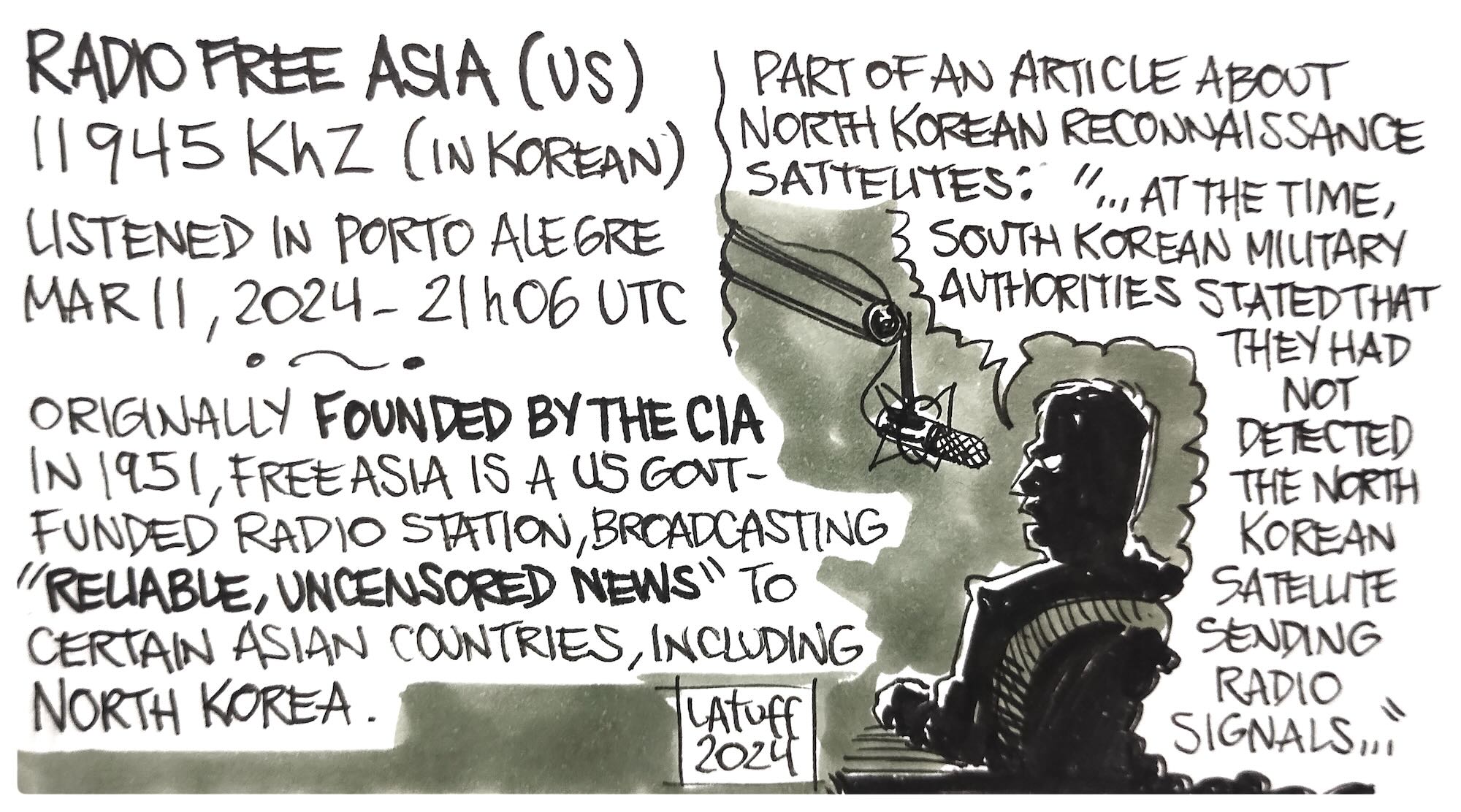
 Many thanks to SWLing Post contributor and noted political cartoonist, Carlos Latuff, who shares this special dive into the world of radio both in and targeting the Korean peninsula. His report includes off-air recordings along with his own original artwork.


 Korean Central Broadcasting Station (KCBS) Pyongyang is the DPRK’s domestic radio station, whose programming reaches North and South Korea, even being heard in Japan. News about the achievements of North Korean leader Kim Jong-un, music and attacks on Seoul government, seen by Pyongyang as a puppet regime.